Bayesian Learning of Graph-Based Interaction Potentials with Applications to Studying Animal Behavior

Bayesian Learning of Graph-Based Interaction Potentials

With Applications to Studying Animal Behavior

Daniel Waxman

Basis Research Institute & MIT

Joint work with

Emily MackeviciusBasis Research Institute

Asilomar

October 27th, 2026

Animal interactions is a signal processing problem

Signal processing fundamentally concerns how information is digested, transformed, and used
Recently, human social dynamics have been a fruitful manifestation of this idea
- But what about animal social interactions?
- How does complex collective behavior arise here?

(Reynolds, 1987)

(Böck et al., 2026)

Animal interactions as a signal processing problem

This problem has attracted lots of attention in applied math, ecology, and statistical physics
This is despite what is — in my opinion — a perfect setting for Bayesian, graph signal processing
We're going to rephrase the common animal interactions problem in a Bayesian SP context
- We'll see what equivalencies fall out
- More importantly, we'll see what new ideas pop out, “for free,” that seem worth exploring

A mathematical view

These systems are a classic interacting particle system
Let \(\mathbf{x}_t=[\mathbf{x}_t^{(1)},\dots,\mathbf{x}_t^{(N)}]\), with \(\mathbf{x}_t^{(n)}\in\mathbb{R}^{d_x}\)
As a starting point, consider systems of the form
\[ \frac{d\mathbf{x}_t^{(n)}}{dt} = \sum_{m\neq n} \Phi_{m\to n}\!\left( \mathbf{x}_t^{(m)},\mathbf{x}_t^{(n)} \right). \]
Given data \(y_{t_1},\dots,y_{t_K}\), we must learn the interaction law \(\Phi_{m\to n}(\cdot,\cdot)\)

Inference requires a simpler model

This is a pretty hopeless problem — we must restrict our model class
A typical restricted model class uses a radially-symmetric interaction, shared for all \(m,n\)
\[ \Phi(\mathbf{x}_m-\mathbf{x}_n) = \phi(r_{nm})(\mathbf{x}_m-\mathbf{x}_n), \qquad r_{nm}=\|\mathbf{x}_m-\mathbf{x}_n\|. \]
This implies a weighted graph, describing interactions: \[ W_{nm}(X)=\phi(r_{nm}). \]

Identifiability guarantees come from stricter assumptions

Much existing literature focuses on identifiability of the interaction kernel
- For example, in a first-order ODE, one may state a coercivity condition (Lu et al., 2019)
- Roughly, perturbations of the kernel must create distinguishable trajectories
- With further assumptions, this gives uniqueness and convergence rates
These assumptions are restrictive! They are not automatically satisfied by our animal data

A different extreme from machine learning

We may also disregard structure more completely
For example, we can use graph neural networks for more black-box predictions
But what about interpretation?!
Also, we just don't have much data! Learning these is hard (Aitsahalia et al., 2025)

Positions aren't always enough

Interactions may also happen on the velocity instead (D’Orsogna et al., 2006)
This is obviously useful in situations where coordinated turning happens
\[ d\mathbf{x}^{(n)}=\mathbf{v}^{(n)}\,dt, \qquad d\mathbf{v}^{(n)}=F_n(X)\,dt. \]
This gives us inertia

Motion isn't completely deterministic, either

We may relax the ODE assumption to an SDE (Ha et al., 2009)
Theoretically, this has interesting consequences
- It corresponds to the McKean-Vlasov PDE line
More generally, though, it is very useful for computation
\[ dX=V\,dt, \qquad dV=F(X)\,dt+\Sigma\,dB_t. \] \[ Y_k=X_{t_k}+\epsilon_k. \]

Animals may also align their velocities

An animal can respond to where its neighbors are
But it can also respond to how they are moving (Cucker & Smale, 2007)

\[ d\mathbf{v}^{(n)} = \left[ F_n(X) + \sum_{m\neq n} \psi(r_{nm}) \left(\mathbf{v}^{(m)}-\mathbf{v}^{(n)}\right) \right]dt +\Sigma_n\,dB_t. \]

What about persistent, social interactions?

So far, every animal interacts with every other animal
But we can also set persistent weights
- This may be thought to model social activities, like parent/kin, etc.
\[ d\mathbf{x}^{(n)} = \sum_{m\neq n} a_{nm}\,\phi(r_{nm}) \left(\mathbf{x}^{(m)}-\mathbf{x}^{(n)}\right)dt +\sigma\,dB_t^{(n)}. \]
Lang et al. (2026) learn graph and dynamics jointly with an alternating least squares

Signal processing as a middle road

As an SP problem, this is a system identification task
The animals carry signals; their interactions process those signals
We want to learn both the graph and the processing rule

These are related to graph diffusions

The processes above are related — but different than — a graph diffusion process
A graph diffusion process uses the graph Laplacian \(L\) of a fixed undirected graph \(W\)
- It posits linear interactions according to the graph
\[ \dot X=-LX, \qquad L=\operatorname{diag}(W\mathbf1)-W. \]
Solutions are solved via the matrix exponential, \[ X_{t+\Delta}=e^{-\Delta L}X_t. \]
We may take a spectral decomposition \(L=U\Lambda U^\top\), so that \[ e^{-\Delta L} = U\,\operatorname{diag}\!\left(e^{-\Delta\lambda_k}\right)U^\top. \]
This is a form of a graph filter
- Similar to how discrete filters modify spectra, graph filters modify \(\Lambda\)

Interacting particles give us a changing graph

Our graph changes dynamically according to \(X\): \[ W_{ij}(X)=a_{ij}\phi(r_{ij}), \qquad L_\phi(X)=\operatorname{diag}(W(X)\mathbf1)-W(X). \]
The familiar interaction model becomes
\[ \dot X=-L_\phi(X)X. \]
This model now captures both static interactions (via \(A\)), and the dynamic interactions (via \(\phi\))

Learning interactions non-parametrically

Interaction kernels are typically learned with basis expansions
- ... that are useful for convergence results
We'll use a Bayesian basis expansion, approximating a Gaussian process \[ \phi(r)=\sum_{m=1}^{M}c_m e_m(r). \]
With a particular prior, this is a Hilbert space Gaussian process (Solin & Särkkä, 2020) \[ c_m = z_m\sqrt{\mathcal S_{3/2}(\omega_m;a,\ell)}, \qquad z_m\sim\mathcal N(0,1). \]
This GP determines the graph filter

Learning the dynamics

We have tremendous tracking difficulties in practice
- But solutions often require perfect observation
We can set a more generic observation model, to determine an SSM
\[ dZ_t=f_\theta(Z_t)\,dt+G_\theta\,dB_t, \qquad Y_k=HZ_{t_k}+\epsilon_k. \]
We can then treat this as a typical Bayesian system identification problem to yield \[ p(\theta\mid Y)\propto p(\theta)\,p(Y\mid\theta), \]

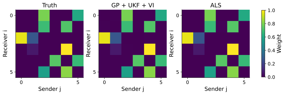
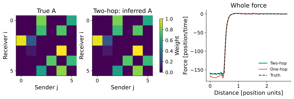
First, can we recover a known graph?

We set up a 2d example from Lang et al. (2026), with a Lennard–Jones-style interaction
Learn the graph and the kernel together

We also recover the interaction law

The HSGP has no particular prior about Lennard-Jones interactions
ALS gets a dictionary prior containing the true interaction
The HSGP still recovers the interaction quite well

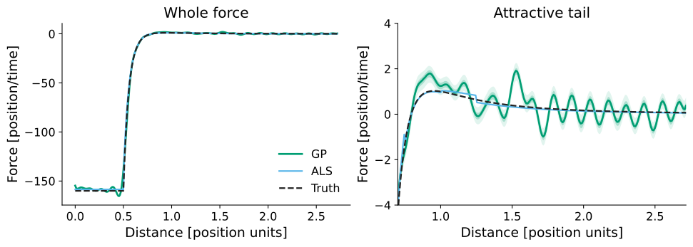
Exploration-weighted force error	HSGP	ALS
	2.62%	2.62%

What does GSP add?

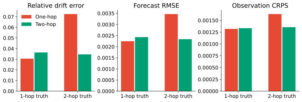
One idea: why stop with one graph filter application? \[ X \xrightarrow{\;-L_\phi(X)\;} u \xrightarrow{\;I-\gamma L_\phi(X)\;} b \] \[ u=-L_\phi(X)X, \qquad b=u-\gamma L_\phi(X)u. \]
Equivalently,
\[ dX= \left[-L_\phi(X)+\gamma L_\phi(X)^2\right]X\,dt +\sigma\,dB_t. \]
An agent now responds to its neighbors’ responses
- We could think of this as a type of coordination

Does the extra hop help when it is really there?

Positions and velocities are two graph signals

The same idea gives us two interaction channels
\[ dX=V\,dt, \] \[ dV= -L_E(X)X\,dt - \left[\alpha P+H(L_A(X))\right]V\,dt +\Sigma\,dB_t. \]
\[ W^E_{ij}=S_{ij}\phi_E(r_{ij}), \qquad W^A_{ij}=S_{ij}g_A(r_{ij}). \]
Positions give us attraction–repulsion & velocities give us alignment

Some encouraging signs in the pigeons

Data: GPS tracks of pigeon flocks (Nagy et al., 2010)
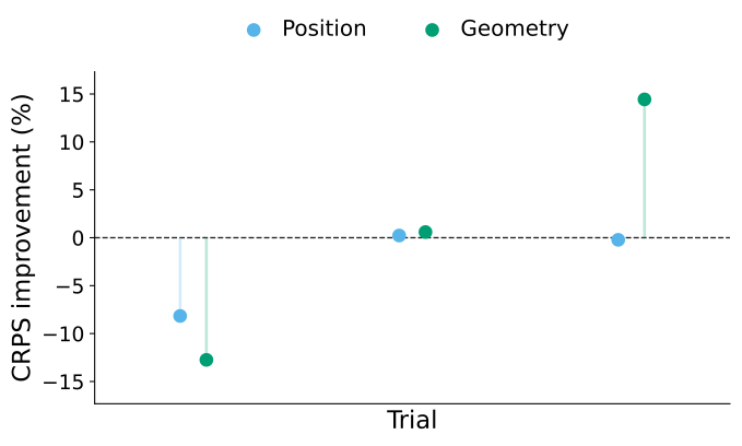
- Three free flights (ff1, ff3, ff11): 8, 7, and 10 birds, 3D positions at 5 Hz
- Fit on 72 observations, then forecast the next 24 (4.8 s); two windows per flight
Interestingly, two-hop dynamics, on some runs, helps geometric CRPS
The results are mixed, but this points to an interesting direction

Flight	Geometry CRPS improvement
ff1	−12.7%
ff3	+0.6%
ff11	+14.4%

Are we learning coordination more than navigation?

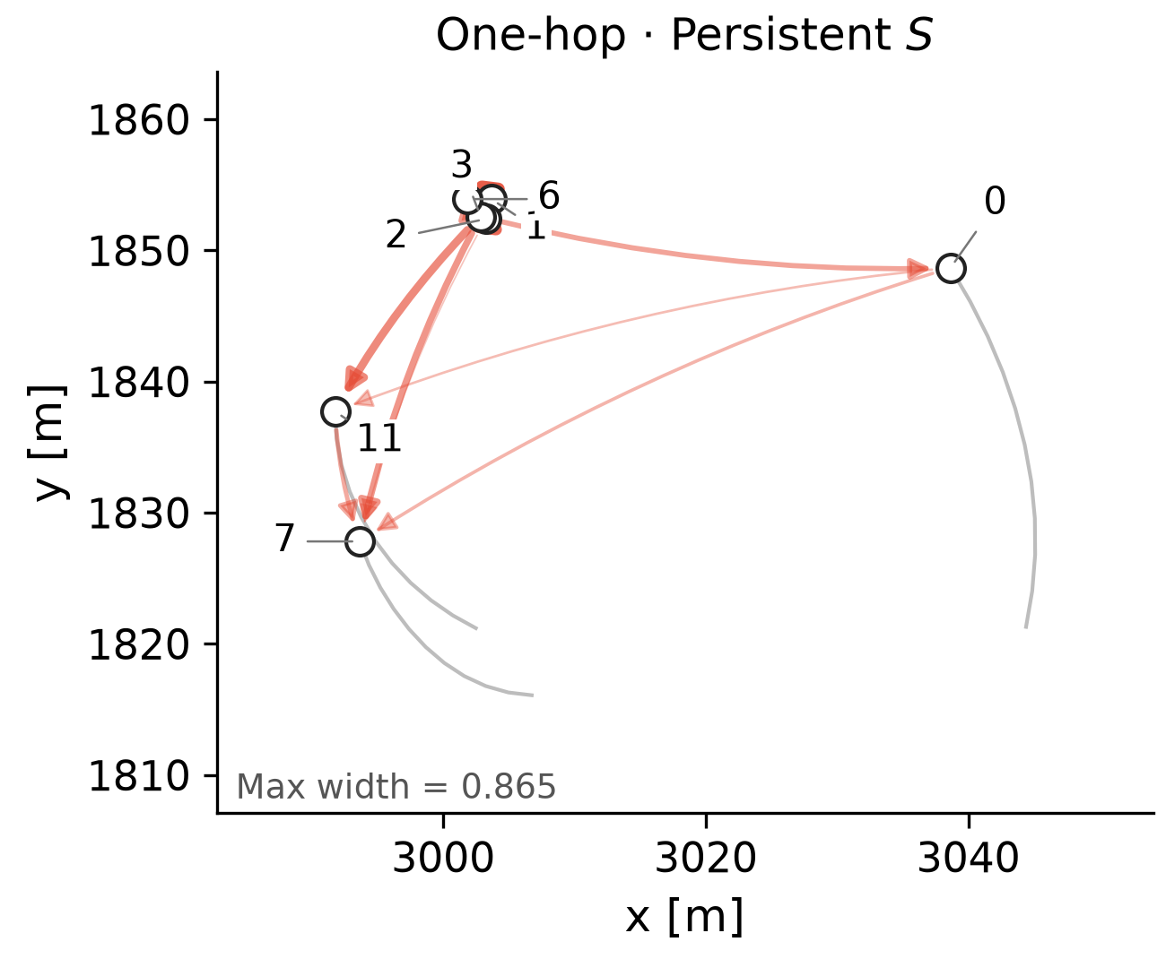
The learned graph gives us other questions to ask

Which animals appear to influence the others?
Do the stronger senders also tend to lead turns?

What's next?

We get a system identification problem on time-varying graphs
This is a problem with meaningful data scarcity, and one where interpretation matters
There are lots of things to explore!
- Do these two-hop models help more broadly?
- Can we develop better particle algorithms?
- How do we deal with the “real” noise pattern?
- Can we interpret things spectrally?

Questions?

danwaxman.github.io

dan@basis.ai