Dynestyx: A probabilistic programming library for dynamical systems

Daniel Waxman

Basis Research Institute & MIT

Joint/ongoing work with

Matthew LevineResearch Scientist
Basis Research Institute

Matthieu DarcyResearch Scientist
Basis Research Institute

Dartmouth ACM Seminar

September 29th, 2026

Who am I

Postdoctoral Fellow @ Basis Research Institute
Research Affiliate @ LIDS, working in the MIT UQ Group
PhD in Electrical Engineering (statistical signal processing) @ Stony Brook University in 2025
Broadly interested in Bayesian stats for dynamical systems

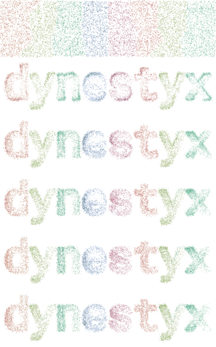
dynestyx is a probabilistic programming library for dynamical systems (DW et al., 2026)
It provides a large suite of state-of-the-art methods for Bayesian inference in dynamical systems
It does this in an interpretable, principled way that enables “Bayesian workflow”

A Brief Motivation of Dynamical Systems

Dynamical systems provide complex systems & structure

Dynamical systems are a natural language for physical and biological systems
Even with simple rules, the results are often complex
The rich structure that yields emergent behavior also yields pathologies

State space models as a formalism

State space models (SSMs) will be our formalism
SSMs consist of a state dynamics process
- Let's write \(x_t \in \mathbb{R}^{d_x}\), where \(t\) can be discrete-time (difference equation) or continuous-time (differential equation)
- In either case, we specify \(x_0 \sim p(x_0)\)
We then observe \(y_t \sim p(y_t \,|\, x_t)\)
- For us, \(y_t \in \mathbb{R}^{d_y}\), always in discrete time

\[ x_t \sim \overbrace{p(x_t \mid x_{t-1})}^{\text{transition density}} \quad\text{or}\quad \mathrm{d}x_t = \overbrace{f(x_t, t)\,\mathrm{d}t}^{\text{drift}} + \overbrace{g(x_t, t)\,\mathrm{d}W_t}^{\text{diffusion}} \]

\[ y_t \sim p(y_t \mid x_t) \]

State space models as a formalism

State space models (SSMs) will be our formalism
SSMs consist of a state dynamics process
- Let's write \(x_t \in \mathbb{R}^{d_x}\), where \(t\) can be discrete-time (difference equation) or continuous-time (differential equation)
- In either case, we specify \(x_0 \sim p(x_0)\)
We then observe \(y_t \sim p(y_t \,|\, x_t)\)
- For us, \(y_t \in \mathbb{R}^{d_y}\), always in discrete time
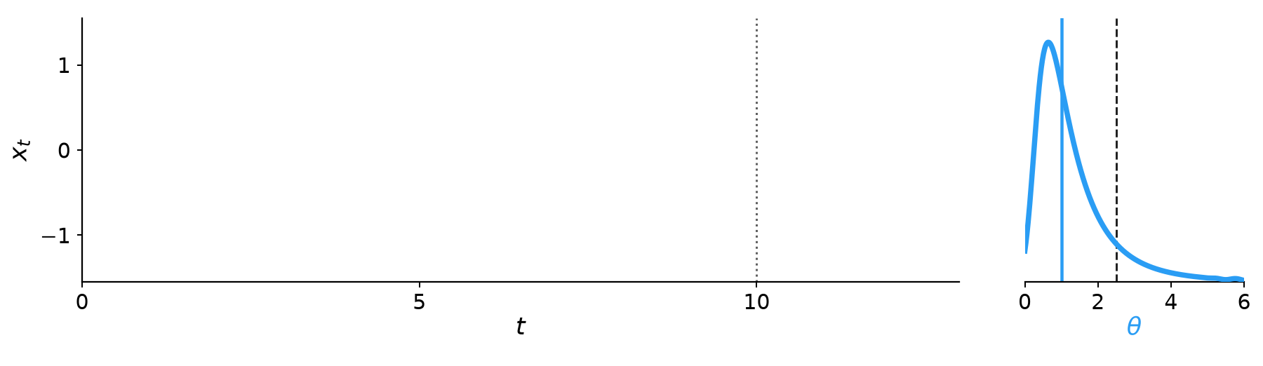
We may additionally parameterize the system by \(\textcolor{#2A9DF4}{\theta} \in \mathbb{R}^{d_{\textcolor{#2A9DF4}{\theta}}}\)

\[ x_t \sim \overbrace{p_{\textcolor{#2A9DF4}{\theta}}(x_t \mid x_{t-1})}^{\text{transition density}} \quad\text{or}\quad \mathrm{d}x_t = \overbrace{f_{\textcolor{#2A9DF4}{\theta}}(x_t, t)\,\mathrm{d}t}^{\text{drift}} + \overbrace{g_{\textcolor{#2A9DF4}{\theta}}(x_t, t)\,\mathrm{d}W_t}^{\text{diffusion}} \]

\[ y_t \sim p_{\textcolor{#2A9DF4}{\theta}}(y_t \mid x_t) \]

ODEs, HMMs, and other special cases

Our generic formulation encompasses other types of systems as special cases
- Ordinary differential equations (ODEs) occur when the diffusion term is identically zero
- Hidden Markov models (HMMs) occur when the state space \(x_t\) is discrete, i.e., \(x_t \in \mathbb{Z}_{H}\)
Some more general classes can also occasionally be written this way
- We can discretize certain PDEs to an ODE or SDE in an appropriate basis

Different inference tasks

There are several different inference tasks we may consider
- Filtering considers the state, given observations up to now: \(p(x_t \,|\, y_{1:t}, \textcolor{#2A9DF4}{\theta})\)
- Smoothing considers the state, given observations past, present, and future: \(p(x_t \,|\, y_{1:T}, \textcolor{#2A9DF4}{\theta}),\ T \geq t\)
- We can also forecast into the future, \(p(x_T \,|\, y_{1:t}, \textcolor{#2A9DF4}{\theta}),\ T \geq t\)
We can learn \(\textcolor{#2A9DF4}{\theta}\) (system identification): \(p(\textcolor{#2A9DF4}{\theta} \,|\, y_{1:T}) \propto p(\textcolor{#2A9DF4}{\theta})\, p(y_{1:T} \,|\, \textcolor{#2A9DF4}{\theta})\)

OU process timeline and prior over theta

Dynestyx

A Probabilistic Programming Language

The “probabilistic programming” part

dynestyx is a library that lets us perform each of these inference tasks
It is a probabilistic programming language (PPL)
- This means it’s like a normal programming language, but the variables are random variables…
- Or in our case, dynamical systems :)
We take a PPL “separation of concerns” seriously: model code describes a mathematical ideal, and all approximations come after

A `dynestyx` model from the ground up

Let’s write our first dynestyx model together; remember, we write down the idealized version
We’ll start by writing down the math, and piece-by-piece, see how this corresponds to code

def model(obs_times=None, obs_values=None, predict_times=None):
    dynamics = dsx.DynamicalModel(

\(x_0 \sim \mathcal{N}(0, 1)\)

        initial_condition=dist.MultivariateNormal(
            jnp.zeros(1), jnp.eye(1)),

\(\mathrm{d}x_t = \sin(x_t)\,\mathrm{d}t + \mathrm{d}W_t\)

        state_evolution=dsx.ContinuousTimeStateEvolution(
            drift=lambda x, u, t: jnp.sin(x),
            diffusion=dsx.ScalarDiffusion(1.0, bm_dim=1),
        ),

\(y_t \sim \mathcal{N}(x_t, 0.1^2)\)

        observation_model=dsx.LinearGaussianObservation(
            H=jnp.eye(1), R=0.1**2 * jnp.eye(1)),

observe \(y_{1:T}\) at \(t_{1:T}\)

    dsx.sample("f", dynamics, obs_times=obs_times,
               obs_values=obs_values, predict_times=predict_times)

A `dynestyx` model from the ground up

def model(obs_times=None, obs_values=None, predict_times=None):

\(\textcolor{#2A9DF4}{\alpha} \sim \mathrm{HalfNormal}(0.5)\)

    alpha = numpyro.sample("alpha", dist.HalfNormal(0.5))

    dynamics = dsx.DynamicalModel(

\(x_0 \sim \mathcal{N}(0, 1)\)

        initial_condition=dist.MultivariateNormal(
            jnp.zeros(1), jnp.eye(1)),

\(\mathrm{d}x_t = \textcolor{#2A9DF4}{\alpha} \sin(x_t)\,\mathrm{d}t + \mathrm{d}W_t\)

        state_evolution=dsx.ContinuousTimeStateEvolution(
            drift=lambda x, u, t: alpha * jnp.sin(x),
            diffusion=dsx.ScalarDiffusion(1.0, bm_dim=1),
        ),

\(y_t \sim \mathcal{N}(x_t, 0.1^2)\)

        observation_model=dsx.LinearGaussianObservation(
            H=jnp.eye(1), R=0.1**2 * jnp.eye(1)),

observe \(y_{1:T}\) at \(t_{1:T}\)

    dsx.sample("f", dynamics, obs_times=obs_times,
               obs_values=obs_values, predict_times=predict_times)

simulate \((\textcolor{#2A9DF4}{\alpha}, x, y) \sim p\)

with dsx.Simulator():
    sim = Predictive(model, num_samples=1)(key, predict_times=ts)

Forking paths of inference

\[ p(\textcolor{#2A9DF4}{\theta} \mid y_{1:T}) \propto p(\textcolor{#2A9DF4}{\theta})\, p(y_{1:T} \mid \textcolor{#2A9DF4}{\theta}) \]

← already hard! classical Bayesian inference

\[ p(y_{1:T} \mid \textcolor{#2A9DF4}{\theta}) = \prod_{k=1}^{T} p(y_k \mid y_{1:k-1}, \textcolor{#2A9DF4}{\theta}) \]

← but where do these come from?

\[ p(y_{1:T} \mid \textcolor{#2A9DF4}{\theta}) = \int \textcolor{#222222}{p(x_0)} \prod_{k=1}^{T} \textcolor{#00897B}{p_\theta(y_k \mid x_k)}\, \textcolor{#E64B35}{p_\theta(x_k \mid x_{k-1})}\, \mathrm{d}x_{0:T} \]

Forking paths of inference

Computation via “unrolling”

One option: we can sample from \(p(\theta, x_{0:T} \mid y_{1:T})\) jointly, then “drop” the \(x_t\) samples
This is a classic trick in Monte Carlo for marginalization!
- e.g., it’s the one we use in slice sampling
This can work well for small problems
But as \(T\) gets large, the Monte Carlo problem is high-dimensional (hard!) and loses structure (less robust!)
In dynestyx, we call this a LatentPathBuilder

with LatentPathBuilder():
    with Discretizer(LocalLinearizationConfig()):
        mcmc = MCMC(NUTS(model), num_warmup=500,
                    num_samples=1_000)
        mcmc.run(key, obs_times, obs_values)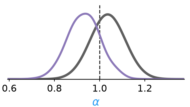

Forking paths of inference

Computation via filtering

\[ p(y_{1:T} \mid \textcolor{#2A9DF4}{\theta}) = \prod_{k=1}^{T} \int \textcolor{#00897B}{p_\theta(y_k \mid x_k)}\, p_\theta(x_k \mid y_{1:k-1})\, \mathrm{d}x_k \]

On the other hand, \(p_\theta(x_t \mid y_{1:t})\) is exactly what the filter computes
We can take expectations with respect to the one-step predictive density!
Thus, we use the filter for an approximate likelihood \(p(y_{1:T} \mid \theta)\)
We can pair this with MCMC like before
- this can be exact marginalization, pseudo-marginal MCMC (Andrieu & Roberts, 2009; Andrieu et al., 2010), or just an approximation :)

with Filter(ContinuousTimeEKFConfig()):
    mcmc = MCMC(NUTS(model), num_warmup=500,
                num_samples=1_000)
    mcmc.run(key, obs_times, obs_values)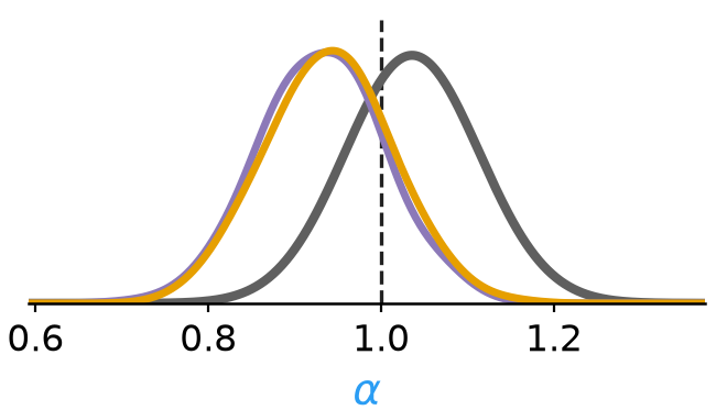

Posterior over alpha, latent path and filter

Forking paths of inference

Variational inference

\[ p(y_{1:T} \mid \textcolor{#2A9DF4}{\theta}) = \prod_{k=1}^{T} \int \textcolor{#00897B}{p_\theta(y_k \mid x_k)}\, p_\theta(x_k \mid y_{1:k-1})\, \mathrm{d}x_k \]

In either case, we can also use variational inference
Related to “variational Bayes with an intractable likelihood” (Tran et al., 2017)

with Filter(ContinuousTimeEKFConfig()):
    guide = AutoNormal(model)
    svi = SVI(model, guide, optax.adam(1e-2),
              loss=Trace_ELBO())
    result = svi.run(key, 2_000, obs_times, obs_values)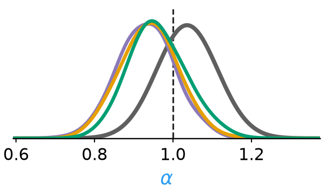

Posterior over alpha, latent path, filter, and variational

Game #1

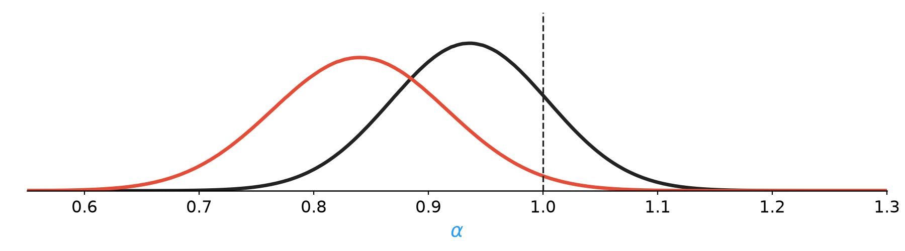
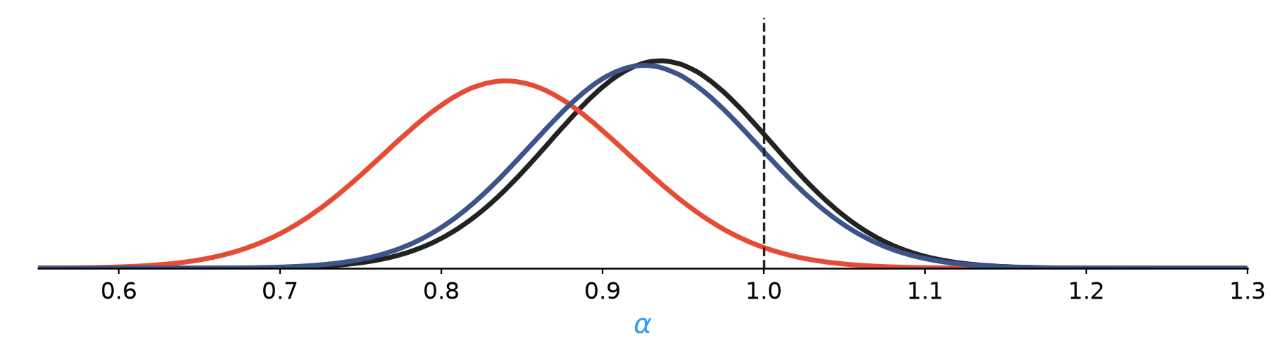
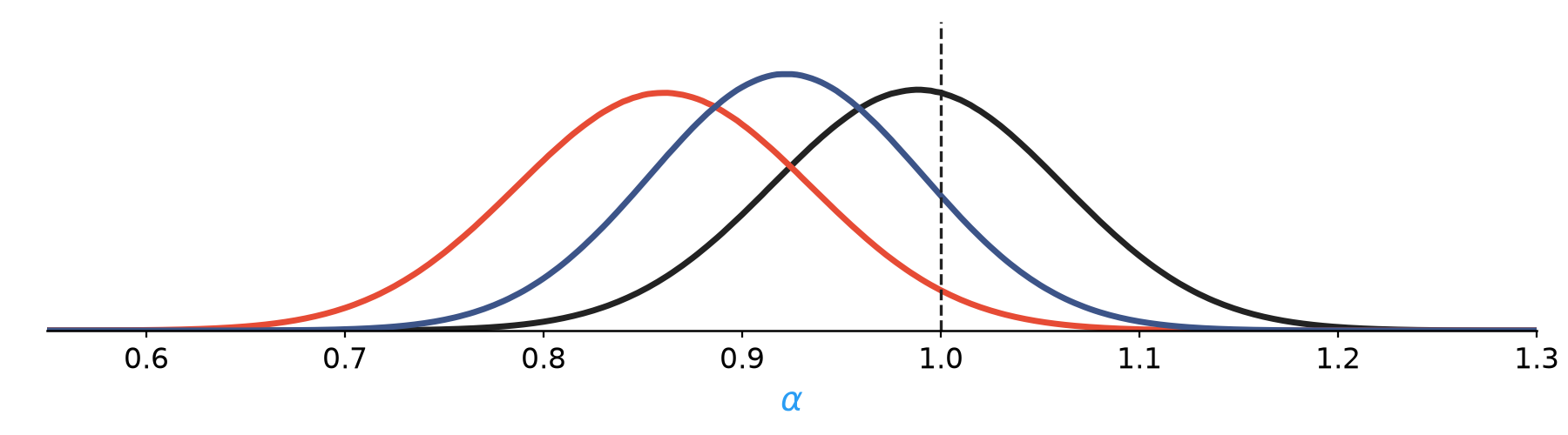
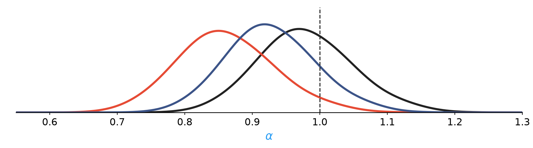
To approximate or to not approximate

To approximate or not to approximate

An example with discretization

Continuous-time EKF

Euler–Maruyama

Local linearization

Ensemble Kalman filter

Variational inference

\(\textcolor{#2A9DF4}{\alpha} \sim \mathrm{HalfNormal}(0.5)\)

\(x_0 \sim \mathcal{N}(0, 1)\)

\(\mathrm{d}x_t = \textcolor{#2A9DF4}{\alpha} \sin(x_t)\,\mathrm{d}t + \mathrm{d}W_t\)

\(y_t \sim \mathcal{N}(x_t, 0.1^2)\)

\(x_{k+1} \mid x_k \sim \mathcal{N}\big(x_k + \textcolor{#2A9DF4}{\alpha} \sin(x_k)\,\Delta t,\; \Delta t\big)\)

\(J_k = \textcolor{#2A9DF4}{\alpha} \cos(x_k)\)

\(x_{k+1} \mid x_k \sim \mathcal{N}\Big(x_k + \tfrac{e^{J_k \Delta t} - 1}{J_k}\, \textcolor{#2A9DF4}{\alpha} \sin(x_k),\; \tfrac{e^{2 J_k \Delta t} - 1}{2 J_k}\Big)\)

with Filter(ContinuousTimeEKFConfig()):
    mcmc = MCMC(NUTS(model), num_warmup=500,
                num_samples=1_000)
    mcmc.run(key, obs_times, obs_values)

with Filter(EKFConfig()):
    with Discretizer(EulerMaruyamaConfig()):
        mcmc = MCMC(NUTS(model), num_warmup=500,
                    num_samples=1_000)
        mcmc.run(key, obs_times, obs_values)

with Filter(EKFConfig()):
    with Discretizer(LocalLinearizationConfig()):
        mcmc = MCMC(NUTS(model), num_warmup=500,
                    num_samples=1_000)
        mcmc.run(key, obs_times, obs_values)

with Filter(ContinuousTimeEnKFConfig()):
    mcmc = MCMC(NUTS(model), num_warmup=500,
                num_samples=1_000)
    mcmc.run(key, obs_times, obs_values)

with Filter(ContinuousTimeEnKFConfig()):
    guide = AutoNormal(model)
    svi = SVI(model, guide, optax.adam(1e-2),
              loss=Trace_ELBO())
    result = svi.run(key, 300,
                     obs_times, obs_values)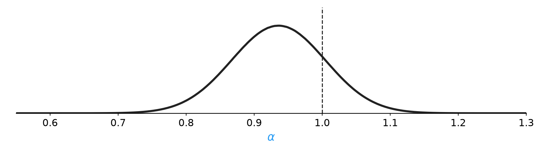

Posterior over alpha with a continuous-time EKF

Posterior over alpha, continuous-time EKF and Euler-Maruyama

Posterior over alpha, continuous-time EKF, Euler-Maruyama, and local linearization

Posterior over alpha with ensemble filters: continuous-time, Euler-Maruyama, and local linearization

Posterior over alpha from SVI: continuous-time, Euler-Maruyama, and local linearization

Game #2

Can we do X?

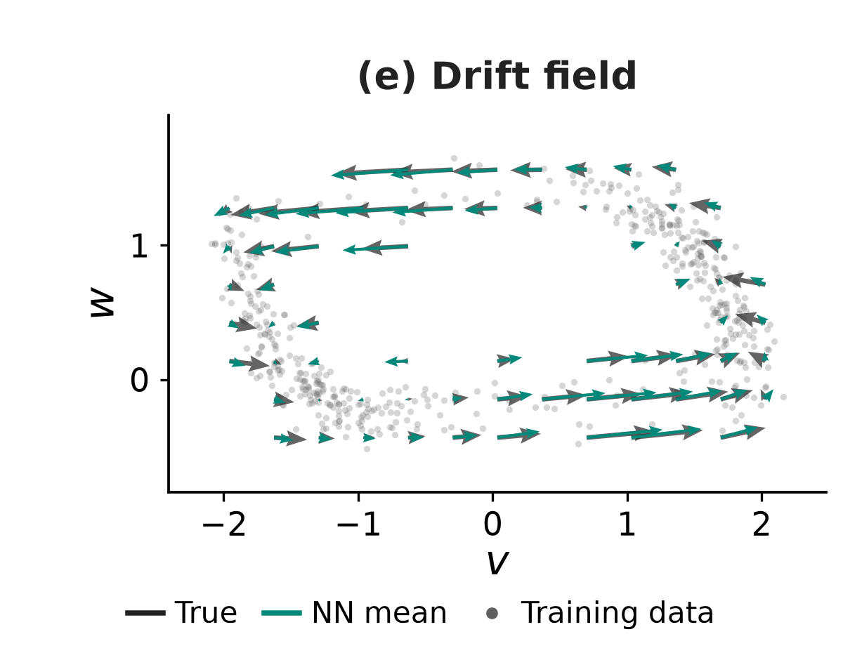
Can we use neural networks?

Yes.

\(\mathrm{d}x_t =\) \((x_t)\,\mathrm{d}t + \sigma\,\mathrm{d}W_t\)

\(y_t \mid x_t \sim \mathcal{N}\!\left(x_t,\,0.01 I_2\right)\)

layers = sample_layers()  # Gaussian priors
dynamics = dsx.ContinuousTimeStateEvolution(
    drift=lambda x, u, t: mlp(layers, x),
    diffusion=dsx.ScalarDiffusion(0.01, bm_dim=2),
)

True FHN drift and final neural-network mean drift near the training observations, shown with a common arrow scale

The code excerpt is from neural_model in python_code/dartmouth_cam_f26/neural_network.py. sample_layers supplies independent Gaussian weight/bias priors; mlp is a 2–16–16–2 tanh network. SVI uses a mean-field Gaussian AutoNormal guide. Each checkpoint filters the same held-out trajectory. Both test observation components are withheld on [10, 15) and [30, 35); training is unchanged. Inside each gap, dynestyx simulates 128 paths per guide draw from the preceding filtered Gaussian. These paths use no later observations. Their covariance and variation across guide draws form the ellipses. The guide stays frozen; ellipses summarize conditional state covariance plus variation across guide draws. The ground-truth model is also filtered using the same approximate continuous-time EnKF. Each panel shows running mean one-step-ahead observation CRPS (lower is better), computed by dynestyx Evaluation with ObservationWiseCRPSScore before assimilating the observation being scored. Scores average both observed components and, for neural models, the 64 frozen-guide draws. Missing observations are excluded from CRPS; its running mean holds constant within each gap. This is the mean conditional Gaussian CRPS, not the CRPS of the mixture over network weights. The right-hand vector field compares true FHN drift with the mean drift over 64 draws of the final guide. It uses a fixed grid restricted to within 0.2 state units of the training observations (gray points). Black and teal arrows share one magnitude scale. FHN setup: https://basisresearch.github.io/dynestyx/stable/deep_dives/gp_drift/

Can we do SINDy?

Yes, we can do (a Bayesian version of) SINDy (Brunton et al., 2016; Hirsh et al., 2022).

theta = numpyro.sample("theta",
    dist.Laplace(0, .1).expand((2, 10)).to_event(2))
dynamics = dsx.ContinuousTimeStateEvolution(
    drift=lambda x, u, t: theta @ library(x),
    diffusion=dsx.ScalarDiffusion(.01, bm_dim=2))

guide = AutoMultivariateNormal(filtered_model, **guide_init)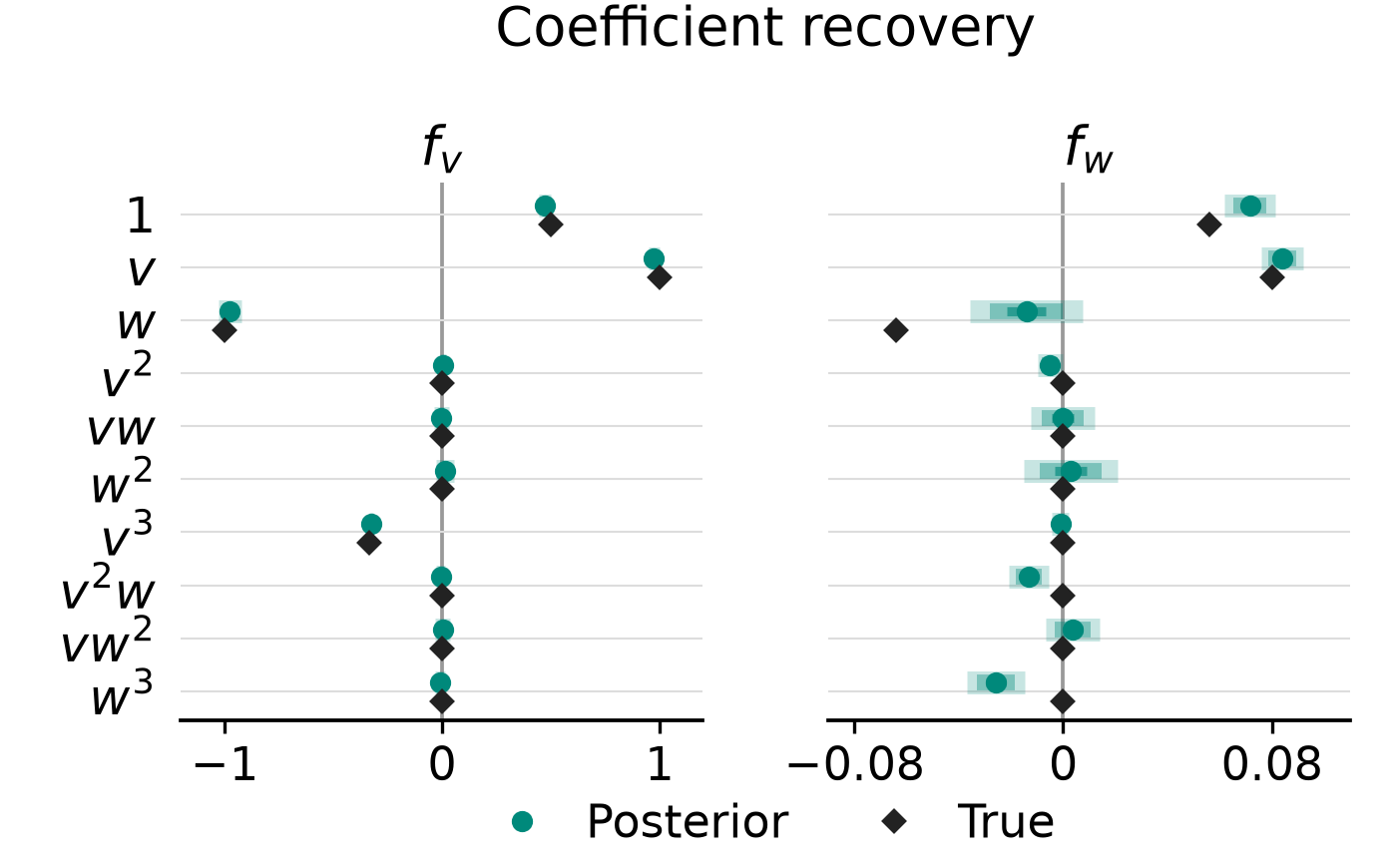

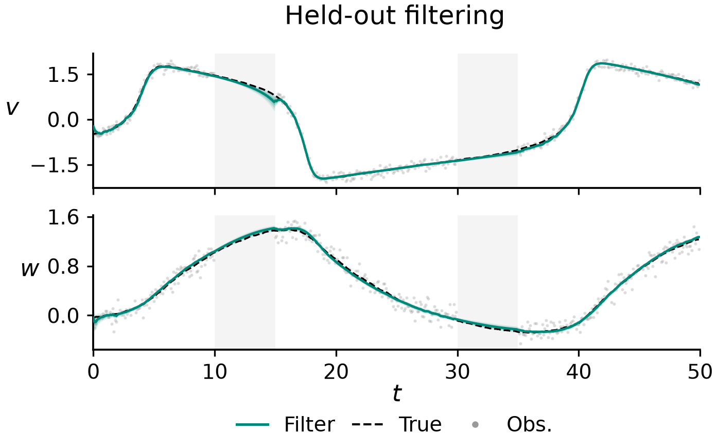
Two horizontal interval plots with shared polynomial term labels: teal posterior means and 50, 80, and 95 percent intervals for all twenty coefficients, compared with black diamond true FHN coefficients

Held-out v and w filtering with truth, available observations and nested uncertainty bands, including two gaps with no observations

Brunton, S. L., Proctor, J. L., & Kutz, J. N. (2016). Discovering governing equations from data by sparse identification of nonlinear dynamical systems. Proceedings of the National Academy of Sciences, 113(15), 3932–3937. https://doi.org/10.1073/pnas.1517384113

Hirsh, S. M., Barajas-Solano, D. A., & Kutz, J. N. (2022). Sparsifying priors for Bayesian uncertainty quantification in model discovery. Royal Society Open Science, 9(2), Article 211823. https://doi.org/10.1098/rsos.211823

This is a Laplace/SVI Bayesian SINDy variant, extending the dynestyx MAP notebook. Hirsh et al. use spike-and-slab or regularized horseshoe priors and MCMC; this is not a reproduction of their algorithm. The SVG shows the matrix-product structure schematically, not fitted support. The polynomial dictionary is fixed. library(x) returns [1,v,w,v²,vw,w²,v³,v²w,vw²,w³]; theta is 2 by 10. No coefficients are thresholded. The executable excerpt comes from sindy.py. The complete model adds the N(0,I) initial condition, Gaussian observation model, dynestyx sample, and continuous-time EnKF handler. guide_init sets zero initial coefficient means and initial scale 0.01. The full Gaussian guide learns correlations. The accepted optimization endpoint is 6,500 steps. Off-slide numerical plumbing retains the notebook's distant-state/derivative safeguard, audited against unguarded filtering. Training uses the neural slide's complete training trajectory. Testing uses its independent trajectory with both components missing on [10,15) and [30,35). The guide remains frozen. Each of 64 coefficient draws runs a conditional filter. Gaps use 128 causal simulated paths per coefficient draw. Bands are 50/80/95 percent marginal Gaussian-mixture quantiles, combining conditional state uncertainty and variation across coefficients. These are pointwise approximate intervals. Coefficient recovery is imperfect: nominal 95% intervals contain 13 of 20 true coefficients. Held-out state RMSE is 0.0352 and mean conditional observation CRPS is 0.0596; the 95% state bands contain 95.0% of latent values in this single held-out trajectory. Reference: https://basisresearch.github.io/dynestyx/stable/deep_dives/fhn_sparse_id/

Can we write hybrid models?

Yes... even for PDEs :)

True system

\(\displaystyle \frac{\partial u}{\partial t}=\nu\frac{\partial^2u}{\partial x^2}+1.1u(1-u)\)

\(x\in(0,1),\quad u(t,0)=u(t,1)=0,\quad \nu=0.01\)

Hybrid model

\(\displaystyle \dot{\mathbf u}=\underbrace{\nu L_h\mathbf u}_{\text{known diffusion}}+\underbrace{\color{#00897B}{c_\theta(\mathbf u)}}_{\text{learned reaction}}\)

\(\mathbf y_k\mid\mathbf u(t_k)\sim\mathcal N\!\left(\mathbf u(t_k),\sigma_y^2 I\right)\)

We learn the missing term with a Gaussian process (GP)
- Specifically, we use a Hilbert space GP (HSGP) approximation (Solin & Särkkä, 2020)

The setup follows the rendered SIAM-NE talk: forty spatial grid points including fixed zero boundaries, thirty-eight interior states, physical diffusivity 0.01, logistic reaction 1.1u(1-u). L_h is tridiag(1,-2,1)/h², with h=1/39. The reaction is one scalar function shared across every node. HSGP means Hilbert-space Gaussian process: a finite Laplacian-eigenfunction approximation. The basis expansion is g(u)=sum_j z_j sqrt(S(alpha,ell;omega_j)) phi_j(u), with c(u)=g(u)-g(0). The HSGP amplitude domain [-1.5,1.5] is distinct from physical space [0,1]. phi_j(u)=sin(omega_j(u+1.5))/sqrt(1.5), omega_j=j*pi/3; S(omega)=alpha² sqrt(2*pi) ell exp(-ell² omega²/2). The zero anchor enforces c(0)=0. Six modes, alpha~HalfNormal(1), ell~LogNormal(log(0.4),0.5), z~N(0,I). Both models infer sigma_y~HalfNormal(0.1); the simulated standard deviation is 0.05. No process noise is included. Hyperparameters and weights are sampled once, outside the ODE drift evaluation. This is a new fit using explicit reproduction defaults, not the old SIAM numerical results.

Can we write hybrid models?

Yes... even for PDEs :)

c = sample_hsgp()  # GP prior for the reaction
dynamics = dsx.ContinuousTimeStateEvolution(
    drift=lambda u, _, t: nu * Lh @ u + c(u))

guide = AutoMultivariateNormal(filtered_model, **guide_init)

The code excerpts are extracted from executable hybrid_pde.py. sample_hsgp samples six standard-normal weights, a squared-exponential amplitude and lengthscale, then returns the centered deterministic callable. nu and Lh are the known diffusion coefficient and finite-difference Laplacian. The complete model includes N(mu0,0.01² I) initial states, inferred Gaussian observation noise, dsx.sample, and the continuous-time EnKF. filtered_model wraps that generative model in Filter; guide_init supplies the agreed initial parameter means and scale. Both models use 32 EnKF particles, fixed filter randomness, and a full-covariance Gaussian parameter guide. Parameters are fitted offline using all eleven training fields from t=0 to 1. The filtering animation reruns causal state updates conditional on this frozen parameter posterior; it is not online parameter learning. The two panels overlay the actual latent truth, not a known-equations filter. Predictions after t=1 receive no observations. Each of 64 parameter draws propagates 128 samples from the full terminal filtered covariance. Bands are pointwise 50/80/95 percent posterior summaries. Cross-state covariance and variation between parameter draws are retained. Displayed guides use 4000 SVI updates each; the user requested rendering before further convergence checks. Forecast RMSE is 0.2856 for diffusion only and 0.01329 for HSGP. The respective inferred observation SDs are 0.1176 and 0.05218, versus the simulated 0.05. These are single-trajectory results, not a calibration study. Numerical results and limitations are recorded in handoff.md.

Can we do hierarchical/mixed-effect inference?

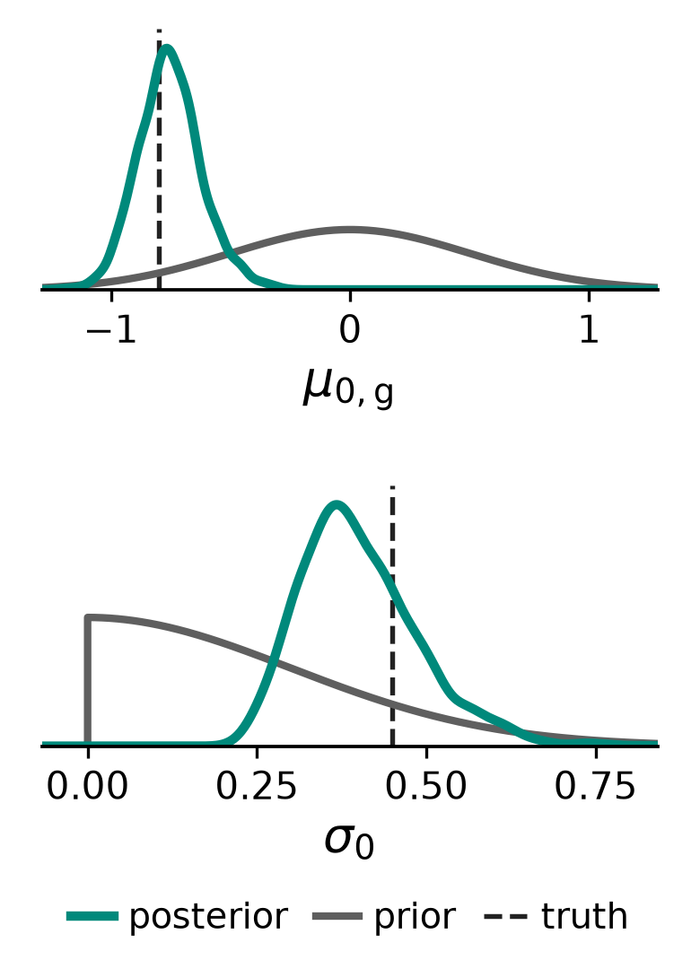
Yes.

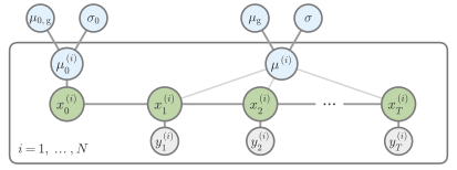
mu0_global = numpyro.sample('mu0_global', dist.Normal(0., .5))
sigma0 = numpyro.sample('sigma0', dist.HalfNormal(.3))
with dsx.plate('individuals', N):
    mu = numpyro.sample('mu', dist.Normal(mu_global, sigma))
    mu0 = numpyro.sample('mu0', dist.Normal(mu0_global, sigma0))
    ou = make_ou(mu, initial_mean=mu0, initial_cov=s0**2)
    return dsx.sample('x', ou, **data)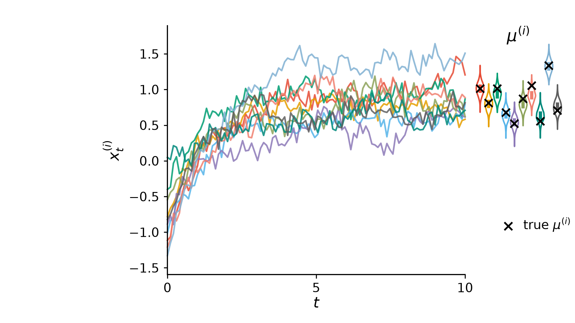

Posterior violins for each agent's OU mean beside the final time, with true means marked

Posterior densities of the population initial mean and scale with truth and prior

Source: https://basisresearch.github.io/dynestyx/stable/tutorials/gentle_intro/08_hierarchical_inference/, reduced to one dimension. Plate diagram: superscript (i) indexes agents, subscript g means global; the OU mean mu^(i) enters every transition (faint edges). Ten agents; dx^(i) = -0.7 (x^(i) - mu^(i)) dt + 0.2 dW, observed every 0.1 with SD 0.08; x_0^(i) ~ N(mu_0^(i), 0.05^2). Priors (shown in the code): mu_g ~ N(0, 0.5^2), sigma ~ HalfNormal(0.4), mu_{0,g} ~ N(0, 0.5^2), sigma_0 ~ HalfNormal(0.3). Truth: mu_g 0.8, sigma 0.3, mu_{0,g} -0.8, sigma_0 0.45. Group scales are SDs. make_ou builds the scalar LTI_continuous model. NUTS with exact continuous-time Kalman likelihoods; mu and mu0 noncentered; two chains of 1000 warmup + 1000 draws, seed 2 (data seed 1); no divergences, R-hat at most 1.008. Posterior medians: mu_g 0.81, sigma 0.26, mu_{0,g} -0.76, sigma_0 0.39, all inside 95% intervals. Violins: posterior for each agent's OU mean (right, x = truth) and initial-condition mean (left, dot = truth), inner bar is the 50% interval. Global panel: posterior KDEs (teal) of the population initial mean and scale, grey prior, dashed truth. Reproduce: python_code/dartmouth_cam_f26/hierarchical.py --run, then --plot.

Other things that can be done

Inference in hidden Markov models (with arbitrary missingness)

Evaluation via proper scoring rules

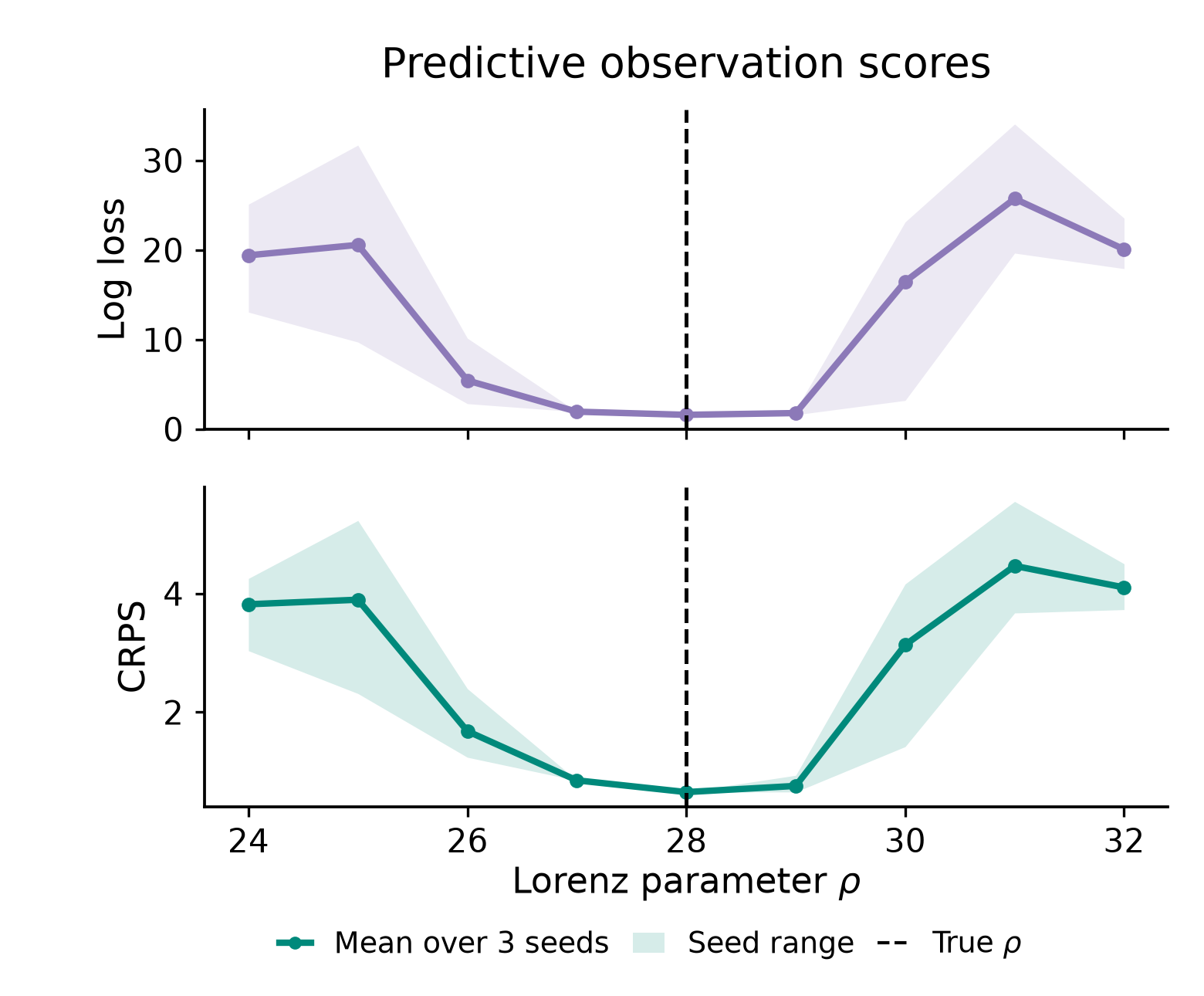
Closed-loop & model-predictive control

More advanced PDEs (Coming soon...)

The bullet and QR code for each topic remain once revealed; the right-hand figure shows only the current topic. HMM: the cited tutorial's two-state correlated Gaussian emissions with whole-field and component-specific missingness. The known transition matrix is fixed; the animation shows exact causal state filtering, not transition-parameter learning. Scores: native dynestyx Evaluation on partially observed Lorenz-63, profiling rho with a 30-particle EnKF. Curves are the mean of three fixed filter seeds; shading is their range, not a posterior interval. Both displayed scores are lower-is-better. Control: the tutorial's linear model and feedback gain, plus a bounded receding-horizon MPC controller driven by the filtered mean. MPC solves an eight-step quadratic objective with controls bounded to [-1,1]; it replans after every observation. Vortex: the existing user-provided vortex_tubes.mp4, illustrating the proposed future PDE capability. Learned localization now has its own slide in the "Learning of filters" section. All QR images link to the supplied tutorial URLs.

New methods

Compositional structure unlocks new methods

Our combinatorial structure unlocks new methods!
Some of these didn’t exist because they’re not good ideas…
But some of them are pretty good!

EnKF-NUTS: Gradient-based ensemble MCMC

Our default method, EnKF with NUTS, is surprisingly good
The pieces are in the literature:
- Ensemble MCMC (Drovandi et al., 2022) uses Metropolis
- Autodifferentiable EnKF (Chen et al., 2022) gives gradients
Our framework allows you to combine these two… along with any other MCMC method or filter you come up with!

EnKF-NUTS performs well

We can compare to particle MCMC, ensemble MCMC, and ensemble NUTS

Sampler	Time	ESS / s	max \(\hat{R}\)	E-BFMI
particle MCMC	113 s	0.16	1.17	–
ensemble MCMC	102 s	11.8	1.01	–
ensemble NUTS	294 s	9.4	1.00	1.02

Stochastic Lorenz-63 observed every 0.1 time units (all components, noise sd 1), one RK4 step (h = 0.1) per observation, T = 100, learning six unknowns: rho, sigma, beta and the initial state x0. Corner plot of rho, sigma, beta and the first coordinate of x0 over an MCMC-free, EnKF-free reference: importance sampling (5000 multivariate-t draws, 1000-particle particle-filter likelihoods, 52 s, IS ESS 1769). Samplers: particle MCMC (1000-particle PF + joint adaptive random-walk Metropolis, warm-started at the posterior because from the shared start it never accepted a move), ensemble MCMC (100-member EnKF + the same random walk, as in Drovandi et al.; 4500 warmup + 9000 draws per chain), ensemble NUTS (same EnKF + NUTS; 500 + 1000). Animation: each sampler's first chain, one after another at real cost (compilation excluded). Table, 4 chains each, worst case over all six unknowns: total time 113 / 102 / 294 s; ESS/s 0.16 / 11.8 / 9.4; max R-hat 1.17 / 1.01 / 1.00; eNUTS E-BFMI min 1.02, no divergences. All three agree with the reference in the mean. With five RK4 substeps NUTS was 2x slower per step (backprop through the integrator) and trailed at 4.5 ESS/s; with one step the two EnKF samplers are comparable. Code: python_code/dartmouth_cam_f26/enkf_nuts.py.

Learning of filters

We can learn parameters of our filters

Often, we have hyperparameters associated with filtering algorithms
In the EnKF, covariance inflation and localization give famous hyperparameters
Recent work has moved towards learning such parameters via autodiff (Adrian et al., 2026)

Learning via proper scoring rules

dynestyx gives an API for proper scoring rules, and is compatible with learning of filters (related to Bach et al., 2026)!

Lorenz-96, 40 states, every other site observed with unit noise; 20-member EnKF with a fixed seed. Two filter hyperparameters are learned jointly: the Gaussian taper radius ell of the covariance localization and the inflation delta. Loss: mean energy score of the one-step predictive observation distribution on cycles 50–199, differentiated through the whole filter; L-BFGS-B in sigmoid-mapped coordinates from ell=11, delta=0.25. Left: the loss surface on a 20×20 grid (colour clipped just above the optimum), with the L-BFGS path. Right: held-out state RMSE on cycles 200–299 (log scale) for each iterate (older iterates fade) against the plain EnKF with neither localization nor inflation (RMSE 4.40; learned 0.26). Inflation alone rescues the unlocalized filter (delta=0.1 gives 0.32), so the baseline is the untuned EnKF. Numbers are in python_code/dartmouth_cam_f26/_cache/learned_filters/diagnostics.json.

Concluding Remarks

Dynestyx is ready-to-use

dynestyx provides the state-of-the-art in inference for practitioners to use, helping to close a gap between theory and application
Algorithms are available for continuous & discrete time, deterministic & stochastic processes
We support control, learning of filters, and lots more
The framework dynestyx creates implies new algorithms, and an avenue for applying new methods

There's lots left to do

Our thesis: closing this gap will uncover a wide array of new methodological work
- Applications will have their own pathologies, and we need methods that effectively detect and address them
We want to provide support to people who want to use dynestyx
- Develop benchmarks based on challenges we see
- Develop diagnostics that can detect pathologies
- Ultimately, use our general framework + knowledge we gain to develop new methods

Questions?

danwaxman.github.io

dwaxman@mit.edu

dynestyx

Paper

GitHub