Online & Predictively-Oriented Model Fusion
Daniel Waxman
Basis Research Institute / MIT
ISBA World Meeting
July 2nd, 2026

Supervised Learning
Training Data
\(x_n, y_n \stackrel{\mathrm{i.i.d.}}{\sim}p(x, y)\)
Machine Learning Model
\(\mathbf{\theta}\)
\(x \sim p(x)\)
\(y | x \sim p(y | x)\)
\(\psi_{\text{EB}} = \mathrm{arg max}_{\psi} p(y \,|\, x, \psi)\)
Online Learning
\(x_5\)
\(x_4\)
\(x_3\)
\(x_1\)
\(x_2\)
\(\def\given{\,\vert\,}\def\V#1{\mathbf{#1}}p(y \given \V{x},\mathcal{D}_4)\)
\(\def\given{\,\vert\,}\def\V#1{\mathbf{#1}}p(y \given \V{x},\mathcal{D}_3)\)
\(\def\given{\,\vert\,}\def\V#1{\mathbf{#1}}p(y \given \V{x},\mathcal{D}_2)\)
\(\def\given{\,\vert\,}\def\V#1{\mathbf{#1}}p(y \given \V{x},\mathcal{D}_0)\)
\(\def\given{\,\vert\,}\def\V#1{\mathbf{#1}}p(y \given \V{x},\mathcal{D}_1)\)
\(\mathbf{\theta_0}\)
ML Model
ML Model
ML Model
ML Model
ML Model
\(\mathbf{\theta_0}\)
\(\mathbf{\theta_4}\)
\(\mathbf{\theta_3}\)
\(\mathbf{\theta_2}\)
\(\mathbf{\theta_1}\)
\(\psi_{\text{ML}} = \mathrm{arg max}_{\psi} p(y \,|\, x, \psi)\)?
Online Model Fusion
There is a Bayesian solution to this problem
It suffers from model mis-specification
We can instead pursue a type of predictively-oriented approach
This special case gives explicit finite-sample guarantees about better performance
Forming Online Ensembles
Bayesian Model Averaging Considered Harmful
Online Bayesian Stacking
Application to Filtering
DW, Llorente, F., & Djuric, P. (2026). Bayesian Ensembling: Insights from Online Optimization and Empirical Bayes. Transactions on Machine Learning Research.
Bayesian Ensembles
The general problem of Bayesian ensembles is to determine an ensemble posterior predictive combining densities \(p_1, \dots, p_K\):
\(p^{\text{ens}}(y_* | x_*, \mathcal{D}) = g(p_1, \dots, p_K) \).
This simplifies significantly if we choose a log-linear or linear ensemble:
\( \log p^{\text{log-lin}}(y_* | x_*, \mathcal{D}) = \sum_{i=1}^K w_i \log p_i(y_* | x_*, \mathcal{D}) \).
\(p^{\text{lin}}(y_* | x_*, \mathcal{D}) = \sum_{i=1}^K w_i p_i(y_* | x_*, \mathcal{D}) \).
We'll focus on the setting with linear ensembles, in online settings.
Bayesian Model Averaging
Bayesian model averaging (BMA) is the most common approach to linear weighting.
BMA weighs each model according to its
\(w_k = \mathrm{Pr}(M_i | \mathcal{D}) \propto p(\mathcal{D} | M_k) p(M_k)\).
In the online setting, we obtain recursive weights via the prequential decomposition of the log-likelihood:
\(\log p(\mathcal{D}_T | M_k) = \sum_{t=1}^T \log p_k(y_t | \mathbf{x}_t, \mathcal{D}_{t-1})\)
\(w_{t+1,k}^{\text{BMA}} \propto w_{t,
k} p_k(y_{t+1} | \mathbf{x}_{t+1}, \mathcal{D}_t)\),
where \(\mathcal{D}_t\) is all data up to and including \((x_t, y_t)\).
BMA Collapses
BMA is simple, and often effective. But it suffers from model mis-specification.
In fact, we can show Bayesian inference is performing
\(R_T = \underbrace{\sum_t \log p_{k^{*}}(y_{t} | \mathbf{x}_t, \mathcal{D}_{t-1})}_{p(\mathcal{D}_T | M_{k^*})} -\sum_t \log\left(\sum_k w_{t, k} p_k(y_t | \mathbf{x}_t, \mathcal{D}_{t-1}) \right),\)
where \(k_*\) is the model with the largest marginal likelihood. Then \(R_T\) is related to an evidence gain in \(M_{k^{*}}\),\( R_T = \log \mathrm{Pr}(M_{k^*} | \mathcal{D}_T) / \mathrm{Pr}(M_{k^*}). \)
Takeaway: BMA performance is closely tied to model selection.BMA Collapses
In fact, we can show this collapse behaves exactly like an online model selection algorithm!
If the posterior probability of the optimal model \(M_{k^*}\) exceeds its prior probability, i.e., \(\mathrm{Pr}(M_{k^*} | \mathcal{D}) \geq \mathrm{Pr}(M_{k^*})\), then \(R_T\) is bounded both above and below,
\(0 \leq R_T \leq -\log \mathrm{Pr}(M_{k^{*}}).\)
Bayesian Stacking
One way to beat BMA is to
Bayesian stacking [Yao et al., BA '18] optimizes weights over a validation set:
\( w^* = \arg \max_{w \in \mathbb{S}^K} \sum_{(\mathbf{x}_n, y_n) \in \mathcal{D}_\text{val}} \log \sum_{k=1}^K w_k p_k(y_n | \mathbf{x}_n, \mathcal{D}_\text{train}) \)
This is a type of predictively-oriented inference [McLatchie et al., 2025].
Predictively-Oriented Inference
To be specific, [McLatchie et al., 2025] revisit the Bayesian posterior in its variational formulation:
\[ \Pi_n^\dagger = \arg\min_{\Pi_n \in \mathcal{P}(\Theta)} \left\{ -\sum_{i=1}^{n} \int \log p_\theta(y_i \mid \mathbf{x}_i)\,\mathrm{d}\Pi_n(\theta) + \mathrm{KL}(\Pi_n\|\Pi) \right\}. \]
But this representation finds the single most parsimonious model in a model class \(P(\Theta)\), under the hypothesis that data come from \(P(\Theta)\)
In cases where mis-specification is present, [McLatchie et al., 2025] propose the predictively-oriented (PrO) posterior:
\[ \Pi_n = \arg\min_{\Pi_n \in \mathcal{P}(\Theta)} \left\{ -\sum_{i=1}^{n} \log \int_{\Theta} p_{\theta}(y_i \mid \mathbf{x}_i, \theta) d\Pi_n(\theta) + \mathrm{KL}(\Pi_n\|\Pi) \right\}. \]
Bayesian Stacking and PrO Inference
In cases where mis-specification is present, [McLatchie et al., 2025] propose the predictively-oriented (PrO) posterior:
\[ \Pi_n = \arg\min_{\Pi_n \in \mathcal{P}(\Theta)} \left\{ -\sum_{i=1}^{n} \log p_{\Pi_n}(y_i \mid \mathbf{x}_i) + \mathrm{KL}(\Pi_n\|\Pi) \right\}. \]
Bayesian stacking is this objective on \(w\), with an improper prior:
\[ w^* = \arg \min_{w \in \mathbb{S}^K} \left\{ -\sum_{i=1}^n \log \underbrace{\sum_{k=1}^K w_k p_k(y_i \mid \mathbf{x}_i,\mathcal{D}_\text{train})}_{p_{\Pi_n}(y_i \mid \mathbf{x}_i)}\right\} \]
We will pursue an online form of the Bayesian stacking objective, which has clear finite-sample guarantees over the Bayesian solution.
Online Bayesian Stacking
For the online scenario, we introduce a
\({w}^* \coloneqq \arg \max_{w\in \mathbb{S}^K} \sum_{t=0}^{T} \log \sum_{k=1}^K w_k p_k(y_{t} | \mathbf{x}_{t}, \mathcal{D}_{1:t-1}).\)
This has been approached in time series settings before, but never for online learning.
We call the resulting problem and its analysis online Bayesian stacking (OBS).
It turns out that its analysis is tractable and classic, by connecting to online portfolio selection.
Portfolio Selection
At each time \(t\), an investor allocates capital across \(K\) assets with weights \(w_t \in \mathbb{S}^K\).
- Each asset produces a return \(r_{k,t}\).
- The investor's wealth thus grows by \(w_t^\top r_t\).
- Goal: choose weights sequentially to perform nearly as well as some comparator, usually the best fixed \(w\) in hindsight.
\(\text{wealth}_T = \prod_{t=1}^{T} w_t^\top r_t \qquad \Longleftrightarrow \qquad \log \text{wealth}_T = \sum_{t=1}^{T}\log(w_t^\top r_t)\)
OPS Algorithms
OPS algorithms come with robust regret guarantees, that guarantee strong performance in adversarial conditions. Let's look at one such algorithm.
\(w_{t+1} = \frac{w_t \odot \exp( \eta r_t / w_t^\top r_t)}{\lVert w_t \odot \exp( \eta r_t / w_t^\top r_t)\rVert_1},\)
Under mild conditions, the regret of this algorithm is bounded.
Furthermore, the regret is sublinear, i.e., its average is decreasing over time.
OPS Algorithms
OPS algorithms come with robust regret guarantees, that guarantee strong performance in adversarial conditions. Let's look at one such algorithm.
\(w_{t+1} = \frac{w_t \odot \exp( \eta r_t / w_t^\top r_t)}{\lVert w_t \odot \exp( \eta r_t / w_t^\top r_t)\rVert_1},\)
where \(\eta\) is a learning rate parameter and \(\odot\) is the element-wise product.
If the gradients are bounded by \(G_\infty\), the regret for a predetermined time \(T\) is bounded by
\(R_T \leq \frac{G_\infty}{\eta} \sqrt{2 T \log K}\)
for some \(\eta > 0\). This is sublinear.
OPS Algorithms
One of the exciting things about this equivalence is that many algorithms exist to provide different bounds! Some variants include
- The Online Newton Step (ONS) algorithm,
which provides
logarithmic regret with bounded gradients. - The dynamic ONS (D-ONS) algorithm, which adapts ONS to non-stationary environments and can beat the BCRP.
- Algorithms with data-dependent regret bounds.
- Algorithms with robust switching regret guarantees.
OBS Performs Well
We begin with a famous toy example to illustrate the effectiveness of OBS.
We consider data from a linear model, where each model is missing input features.
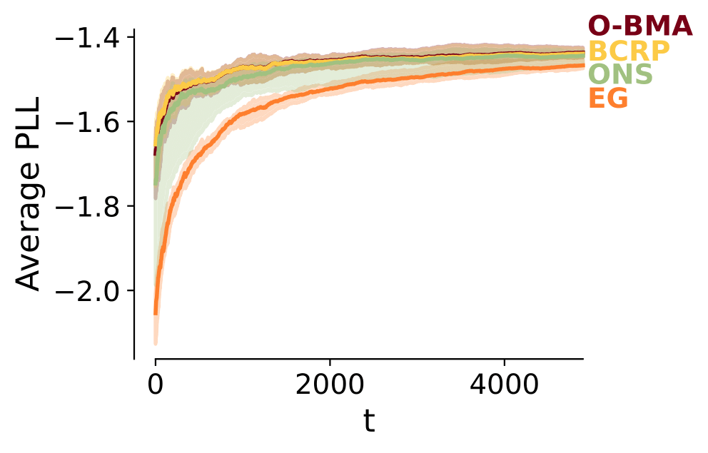
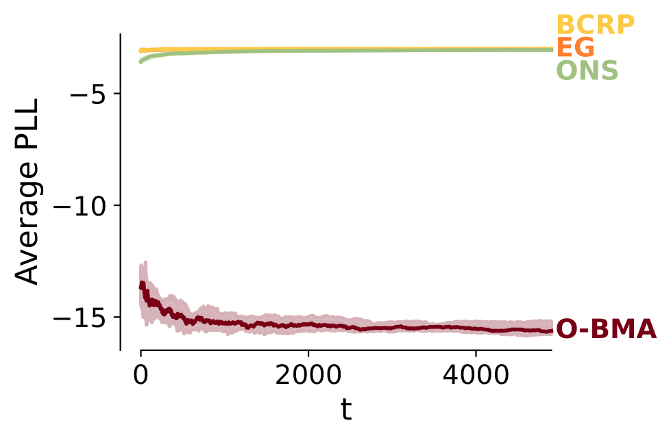
True model included
True model not included
OBS Performs Well
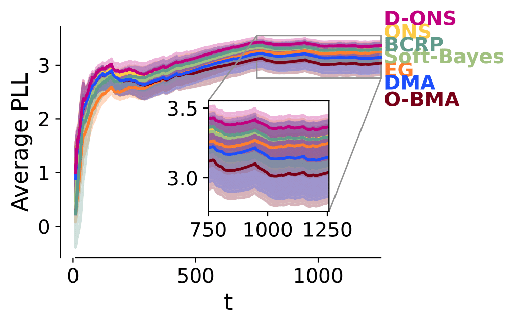
Similar results hold in real, non-trivial Bayesian machine learning settings.
For brevity, here we consider two settings: online variational inference on MNIST, and an online stochastic volatility inference using a variety of GARCH models and sequential Monte Carlo.
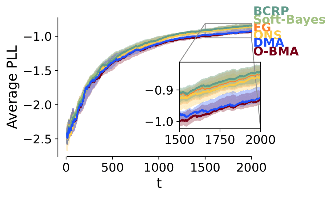
BONG:
Online Bayesian NNs
GARCH:
Online Forecasting
Weights Converge
Weights additionally appear to sensibly converge.
GARCH
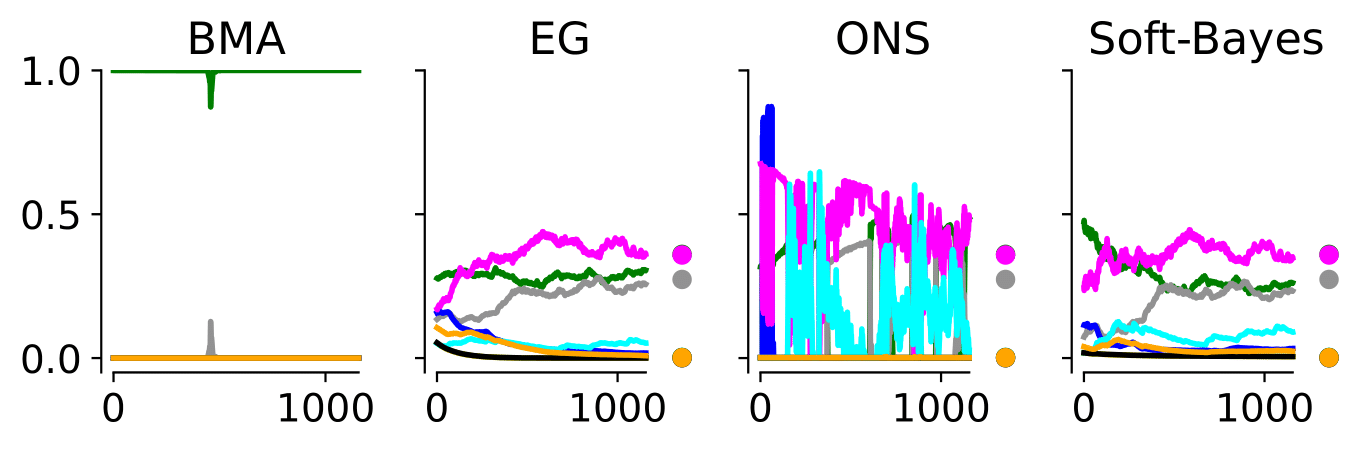
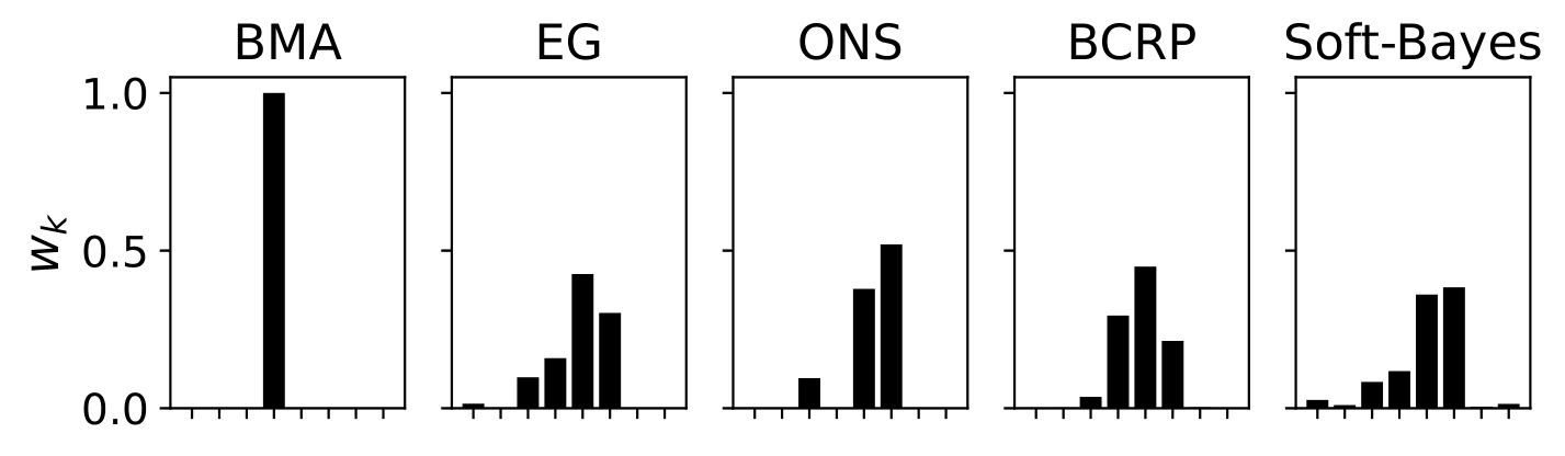
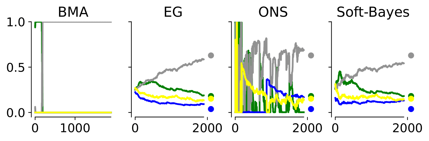
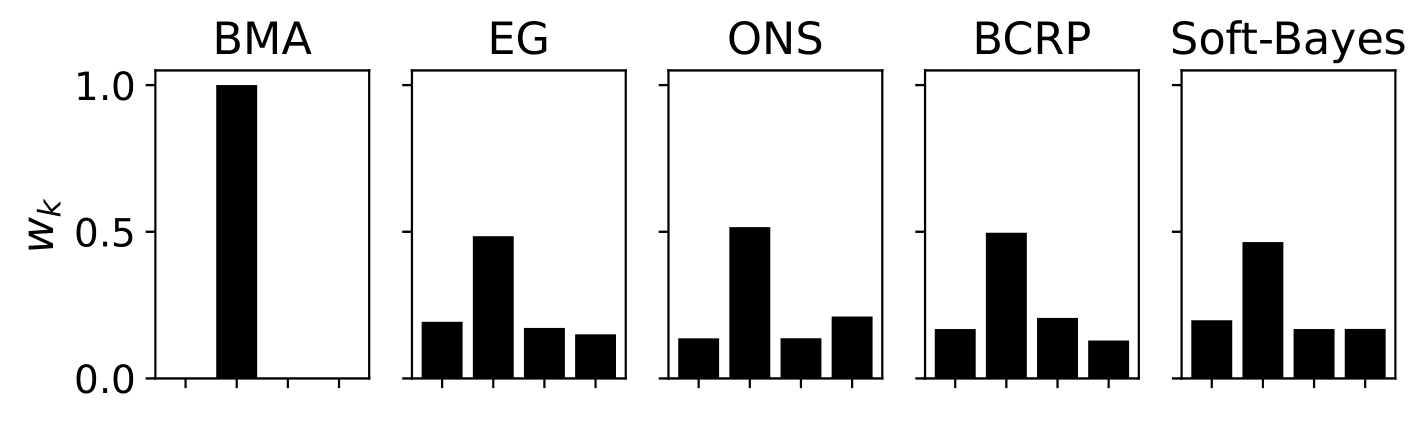
BONG
Application to Filtering
Essentially all of these online Bayesian models amount to some sort of filtering algorithm.
Filtering algorithms use sequential Bayesian inference to update posteriors as new observations \(y_t\) arrive.
As OBS provides
Application to Filtering: Bank of Filters
In a static multiple-model (bank-of-filters) setup, each model/filter \(k\) provides \(p^{(k)}(x_t \mid y_{1:t})\), and we fuse them as
\( p(x_t \mid y_{1:t}) = \sum_{k=1}^K w_{t,k}\, p^{(k)}(x_t \mid y_{1:t}). \)
Classically, bank-of-filters uses BMA-like model probabilities (O-BMA), updated by one-step predictive likelihoods:
\( w^{\mathrm{BMA}}_{t,k} \propto w^{\mathrm{BMA}}_{t-1,k}\, p^{(k)}(y_t \mid y_{1:t-1}). \)
OBS keeps this same bank-of-filters fusion form, but replaces the BMA-style weights with online-optimized weights.
Application to Filtering: IMM and OBS-IMM
This leads to obvious applications on existing algorithms; for example, interacting multiple model (IMM) filters approximate Markov switching:
\( \mu^{i\to j}_{t-1} = \frac{\pi_{ij}\,\mu^{(i)}_{t-1|t-1}} {\sum_{\ell=1}^K \pi_{\ell j}\,\mu^{(\ell)}_{t-1|t-1}} \)
\( \bar p^{(j)}(x_{t-1}\mid y_{1:t-1}) = \sum_{i=1}^K \mu^{i\to j}_{t-1}\, p^{(i)}(x_{t-1}\mid y_{1:t-1}) \)
Vanilla IMM then updates model probabilities in a BMA-like way:
\( \mu^{(j)}_{t|t} \propto \mu^{(j)}_{t|t-1}\, p^{(j)}(y_t\mid y_{1:t-1}). \)
OBS-IMM variant: keep IMM mixing/moment-matching intact, but replace this BMA-like probability update with an OBS update over \(\{p^{(j)}(y_t\mid y_{1:t-1})\}_{j=1}^K\).
OBS-IMM Results
This results in strong performance, and provable theory under model mis-match.
For example, OBS-IMM is superior when we generate data from a Lorenz 63 system and learn neural network drifts.

A Theoretical Problem PrO Filtering
This is exciting! But we shouldn't be too hasty; theoretical analysis of OBS-IMM reveals a pernicious question:
This question underpins the utility of other applications, such as predictively-oriented Kalman filtering [Shen et al., 2026].
Summary
Online Bayesian inference is a practical problem that shows up in lots of contexts, with difficult-to-answer hyperparameter optimization problems.
A common way to cope is to adapt online models with different hyperparameters, and fuse/ensemble them.
The Bayesian approach is well-known, but suffers from extreme model mis-specification. We can provably show it behaves unintuitively and poorly!
We introduce a predictively-oriented version; this comes with simple and robust performance guarantees over the Bayesian solution.
Questions?
danwaxman.github.io
dan@basis.ai