Online Bayesian Learning and Ensembles
Daniel Waxman
Basis Research Institute
Queens for Computing Colloquium
February 9th, 2026

Online Bayesian Learning and Ensembles (with Sequential Bayes)
Daniel Waxman
Basis Research Institute
February 9th, 2026
Supervised Learning
Training Data
\(x_n, y_n \stackrel{\mathrm{i.i.d.}}{\sim}p(x, y)\)
Machine Learning Model
\(\mathbf{\theta}\)
\(x \sim p(x)\)
\(y | x \sim p(y | x)\)
Supervised Learning
Training Data
\(x_n, y_n \stackrel{\mathrm{i.i.d.}}{\sim}p(x, y)\)
Machine Learning Model
\(\mathbf{\theta}\)
\(x \sim p'(x)\)
\(y | x \sim p(y | x)\)
Supervised Learning
Training Data
\(x_n, y_n \stackrel{\mathrm{i.i.d.}}{\sim}p(x, y)\)
Machine Learning Model
\(\mathbf{\theta}\)
\(x \sim p'(x)\)
\(y | x \sim\) \(p'(y | x)\)
Online Learning
\(x_5\)
\(x_4\)
\(x_3\)
\(x_1\)
\(x_2\)
\(y_5\)
\(y_4\)
\(y_3\)
\(y_1\)
\(y_2\)
\(\mathbf{\theta_0}\)
ML Model
ML Model
ML Model
ML Model
ML Model
\(\mathbf{\theta_0}\)
\(\mathbf{\theta_4}\)
\(\mathbf{\theta_3}\)
\(\mathbf{\theta_2}\)
\(\mathbf{\theta_1}\)
Outline
1. Overview of Gaussian Processes
2. Online Bayesian Stacking
3. Online Ensembles of Gaussian Processes
4. How to Implement These Things?
Gaussian Processes
Definitions and Intuitions
Computation Using Kernels
Model Selection
Gaussian Processes
Gaussian Processes: Definitions
Gaussian processes (GPs) are a flexible, non-parametric tool for Bayesian ML. [Rasmussen and Williams, MIT Press '05]
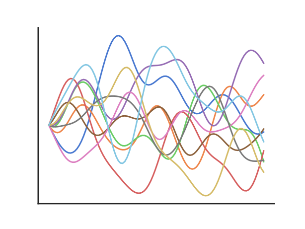
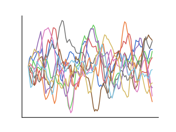
Basic Idea: A GP is a stochastic process \(f_t\) for \(t \in \mathcal{T}\) such the function evaluated at any set of points is jointly Gaussian.
A GP may then be specified by its mean function \( \mu(t) \) and covariance (or kernel) function \( k(t, t') \):
More ML-Like: the paths of any realization of a GP specify a prior over functions.
Gaussian Processes: Computation
In GP regression, we receive data \(t_i, y_i\), with \(i = 1, \ldots, n\), which are noisy observations of \(f(t)\).
\(f \sim \mathcal{GP}\!(0, k)\)
\(y = f(t) + \varepsilon\)
If \(\varepsilon\) is Gaussian, then the posterior is another GP. The posterior predictive is then
\(f_* \mid \mathcal{D} \sim \mathcal{N}(\mu_*, \sigma_*^2)\),
where the mean and the variance are given by
\(\mu_* = \mu(t_*) + k_{* \odot} K_{\odot \odot}^{-1} \delta\),
\(\sigma_*^2 = k(t_*, t_*) - k_{* \odot} K_{\odot \odot}^{-1} k_{* \odot}\).
Symbols
\([K_{\odot \odot}]_{ij} = k(t_i, t_j)\)Training Cross-Covariance
\([k_{* \odot}]_{i} = k(t_*, t_i)\)
Test Cross-Covariance
\(\delta = y - \mu(t)\)
Training Residuals
Gaussian Processes: Computation
In GP regression, we receive data \(t_i, y_i\), with \(i = 1, \ldots, n\), which are noisy observations of \(f(t)\).
\(f \sim \mathcal{GP}\!(0, k)\)
\(y = f(t) + \varepsilon\)
If \(\varepsilon\) is Gaussian, then the posterior is another GP. The posterior predictive is then
\(f_* \mid \mathcal{D} \sim \mathcal{N}(\mu_*, \sigma_*^2)\),
where the mean and the variance are given by
\(\mu_* = \mu(t_*) + k_{* \odot}\) \(K_{\odot \odot}^{-1}\) \(\delta\),
\(\sigma_*^2 = k(t_*, t_*) - k_{* \odot}\) \(K_{\odot \odot}^{-1}\) \(k_{* \odot}\).
Symbols
\([K_{\odot \odot}]_{ij} = k(t_i, t_j)\)Training Cross-Covariance
\([k_{* \odot}]_{i} = k(t_*, t_i)\)
Test Cross-Covariance
\(\delta = y - \mu(t)\)
Training Residuals
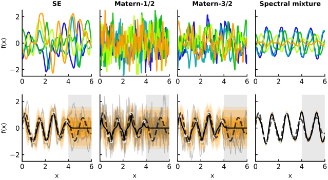
Gaussian Processes: Kernels
Gaussian Processes: Model Selection
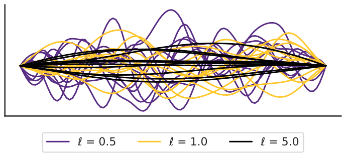
Even after specifying the form of \(\kappa(t, t')\), there are still many choices to be made.
In particular, each kernel comes with a set of hyperparameters which must also be selected.
The typical way to accomplish this with GPs is to maximize the marginal likelihood:
\(\log p(y | \theta) = \log \int p(y | f, \theta) p(f | \theta) \, df\)
Basic Idea: Choose priors that predict the data well.
Gaussian Processes: Ensembles
In (offline) supervised learning, we optimize the marginal likelihood.
In online analysis, optimization is hard.
We will instead focus on forming ensembles over different hyperparameters.
Forming Online Ensembles
Outline
Online Bayesian Stacking
Application to Filtering
Bayesian Ensembles
The general problem of Bayesian ensembles is to determine an ensemble posterior predictive combining densities \(p_1, \dots, p_K\):
\(p^{\text{ens}}(y_* | x_*, \mathcal{D}) = g(p_1, \dots, p_K) \).
This simplifies significantly if we choose a log-linear or linear ensemble:
\( \log p^{\text{log-lin}}(y_* | x_*, \mathcal{D}) = \sum_{i=1}^K w_i \log p_i(y_* | x_*, \mathcal{D}) \).
\(p^{\text{lin}}(y_* | x_*, \mathcal{D}) = \sum_{i=1}^K w_i p_i(y_* | x_*, \mathcal{D}) \).
We will focus on selecting linear weights, though we have also explored how to select log-linear weights for GPs [Ajirak, DW, et al., Asilomar '23].
Bayesian Model Averaging
Bayesian model averaging (BMA) is the most common approach to linear weighting.
BMA weighs each model according to its
\(w_i = \mathrm{Pr}(M_i | \mathcal{D}) = \frac{p(M_i | \mathcal{D}) p(M_i)}{\sum_{j=1}^K p(M_j | \mathcal{D}) p(M_j)}\).
In the online setting, we obtain recursive weights via the prequential decomposition of the log-likelihood:
\(w_{t+1,k}^{\text{BMA}} = \frac{ w_{t, k} p_k(y_{t+1} | \mathbf{x}_{t+1}, \mathcal{D}_t)}{\sum_k w_{t, k} p_k(y_{t+1} | \mathbf{x}_{t+1}, \mathcal{D}_t)}\).
BMA Collapses
BMA is simple, and often effective. However, it does a poor job of
We can show this explicitly in the online setting.
\(R_T = \sum_t \log p_{k^{*}}(y_{t} | \mathbf{x}_t, \mathcal{D}_{t-1}) -\sum_t \log\left(\sum_k w_{t, k} p_k(y_t | \mathbf{x}_t, \mathcal{D}_{t-1}) \right),\)
where \(k_*\) is the model with the largest marginal likelihood. Then \(R_T\) is related to an evidence gain in \(\mathcal{M}_{k^{*}}\),\( R_T = \log \mathrm{Pr}(\mathcal{M}_{k^*} | \mathcal{D}_T) / \mathrm{Pr}(\mathcal{M}_{k^*}). \)
Takeaway: BMA performance is closely tied to model selection.BMA Collapses
In fact, we can show this collapse behaves exactly like an online model selection algorithm!
If the posterior probability of the optimal model \(\mathcal{M}_{k^*}\) exceeds its prior probability, i.e., \(\mathrm{Pr}(\mathcal{M}_{k^*} | \mathcal{D}) \geq \mathrm{Pr}(\mathcal{M}_{k^*})\), then \(R_T\) is bounded both above and below,
\(0 \leq R_T \leq -\log \mathrm{Pr}(\mathcal{M}_{k^{*}}).\)
Bayesian Stacking
One way to beat BMA is to
Bayesian stacking [Yao et al., BA '18] optimizes weights over a validation set:
\( w^* = \arg \max_{w \in \mathbb{S}^K} \sum_{n=1}^N \log \sum_{k=1}^K w_k p_k(y_n | \mathbf{x}_n, \mathcal{D}) \)
In the offline setting, this can be solved efficiently using leave-one-out cross-validation...
... but what if we want to solve for the weights online?
Online Bayesian Stacking
For the online scenario, we introduce a
\({w}^* \coloneqq \arg \max_{w\in \mathbb{S}^K} \sum_{t=0}^{T} \log \sum_{k=1}^K w_k p_k(y_{t} | \mathbf{x}_{t}, \mathcal{D}_{1:t-1}).\)
This has been approached in time series settings before, but never for online learning.
We call the resulting problem and its analysis online Bayesian stacking (OBS).
OBS is Portfolio Selection
The resulting optimization problem turns out to be exactly equivalent to a well-studied problem in finance and online convex optimization!
The Online Portfolio Selection (OPS) Problem
An investor may invest in \(K\) different assets. At each day, she may reallocate her portfolio, at no cost, with the goal to maximize profits.
On day \(t\), stock \(k\) obtains returns \(r_{k, t}\), i.e., the stock is \(r_{k, t}\) times more valuable than at the start of the day.
If \(w_t \in \mathbb{S}^K\) is the investor's portfolio, then their wealth increases by \(w_t^T r_t\) at the end of day \(t\).Their total wealth is thus
\(\text{wealth}_T = \Pi_{t=1}^T w_t^T r_t. \equiv \log \text{wealth}_T = \sum_{t=1}^T \log w_t^T r_t.\)
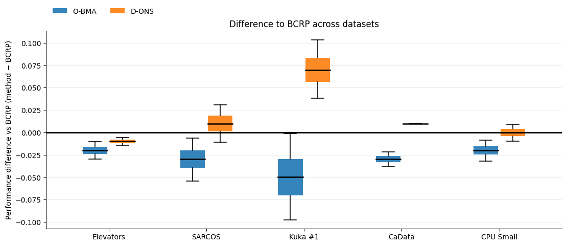
The investor thus seeks to beat the best possible portfolio with a fixed, static \(w\), known as the best constantly rebalanced portfolio (BCRP).
OPS Algorithms
OPS algorithms come with robust regret guarantees, that guarantee strong performance in adversarial conditions. Let's look at one such algorithm.
\(w_{t+1} = \frac{w_t \odot \exp( \eta r_t / w_t^\top r_t)}{\lVert w_t \odot \exp( \eta r_t / w_t^\top r_t)\rVert_1},\)
Under mild conditions, the regret of this algorithm is bounded.
Furthermore, the regret is sublinear, i.e., its average is decreasing over time.
OPS Algorithms
OPS algorithms come with robust regret guarantees, that guarantee strong performance in adversarial conditions. Let's look at one such algorithm.
\(w_{t+1} = \frac{w_t \odot \exp( \eta r_t / w_t^\top r_t)}{\lVert w_t \odot \exp( \eta r_t / w_t^\top r_t)\rVert_1},\)
where \(\eta\) is a learning rate parameter and \(\odot\) is the element-wise product.
If the gradients are bounded by \(G_\infty\), the regret for a predetermined time \(T\) is bounded by
\(R_T \leq \frac{G_\infty}{\eta} \sqrt{2 T \log K}\)
for some \(\eta > 0\). This is sublinear.
OPS Algorithms
One of the exciting things about this equivalence is that many algorithms exist to provide different bounds! Some variants include
- The Online Newton Step (ONS) algorithm,
which provides
logarithmic regret with bounded gradients. - The dynamic ONS (D-ONS) algorithm, which adapts ONS to non-stationary environments and can beat the BCRP.
- Algorithms with data-dependent regret bounds.
- Algorithms with robust switching regret guarantees.
OBS Performs Well
We begin with a famous toy example to illustrate the effectiveness of OBS.
We consider data from a linear model, where each model is missing input features.
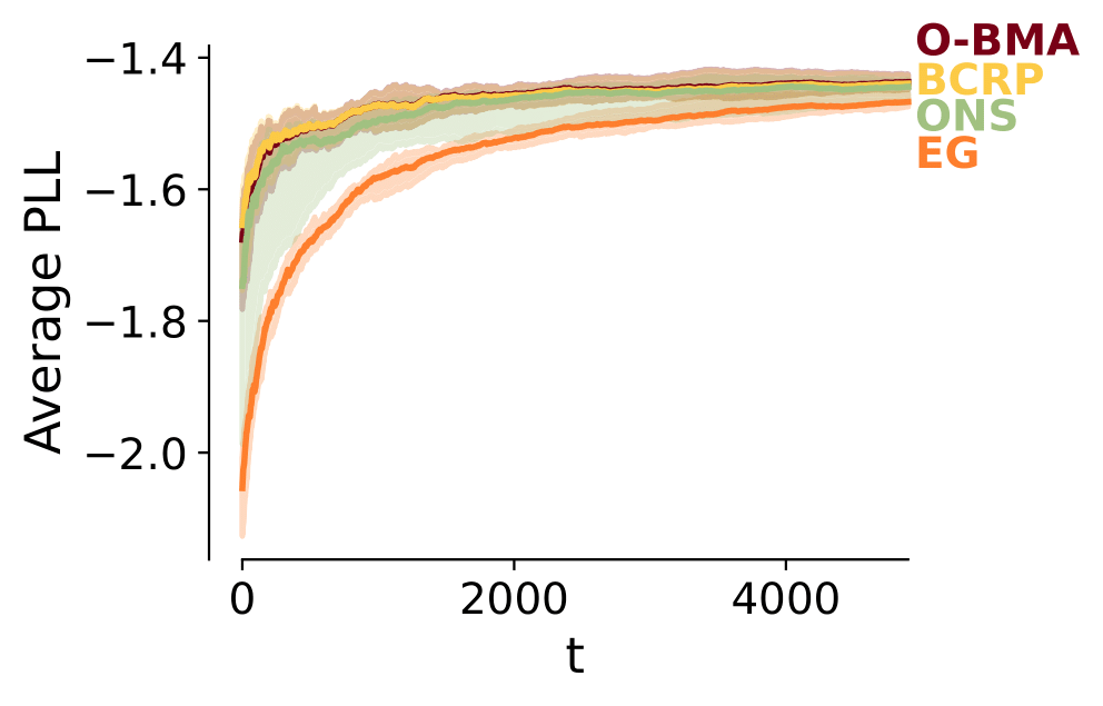
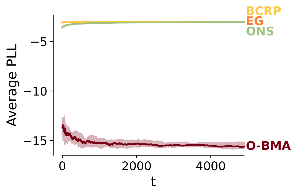
M-Closed:
True model included
M-Open:
True model not included
OBS Performs Well
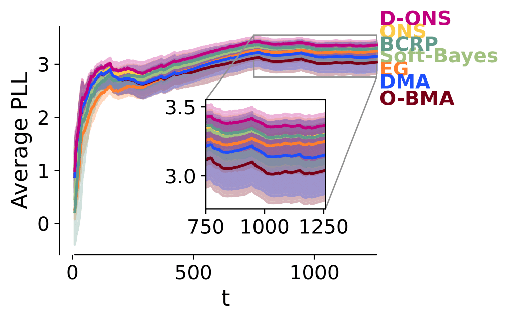
Similar results hold in real, non-trivial Bayesian machine learning settings.
For brevity, here we consider two settings: online variational inference on MNIST, and an online forecasting task using a variety of GARCH models and sequential Monte Carlo.
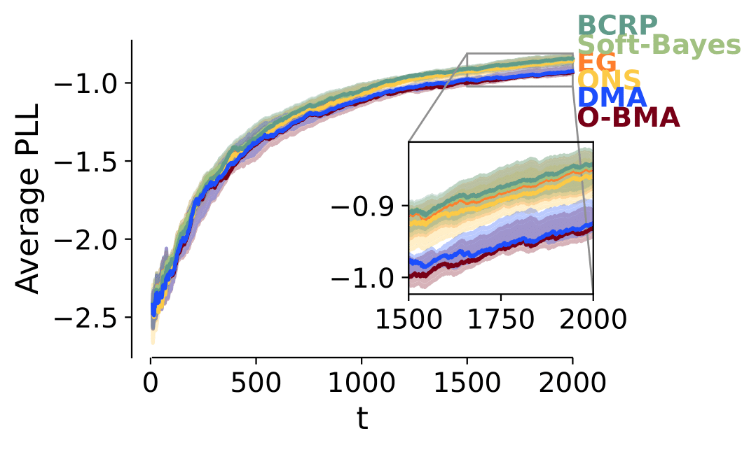
BONG:
Online Bayesian NNs
GARCH:
Online Forecasting
Weights Converge
Weights additionally appear to sensibly converge.
GARCH
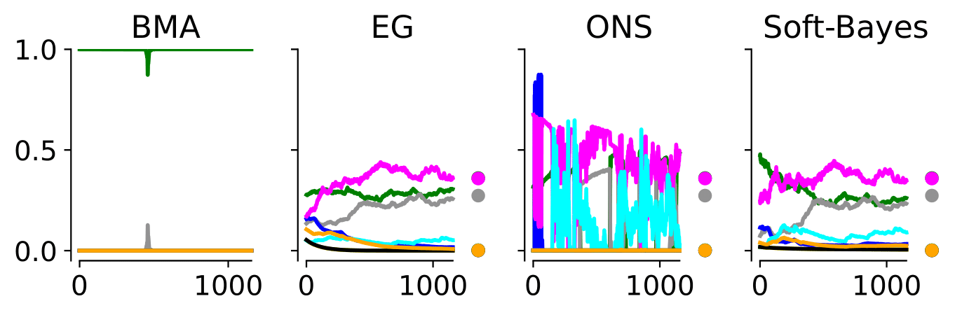
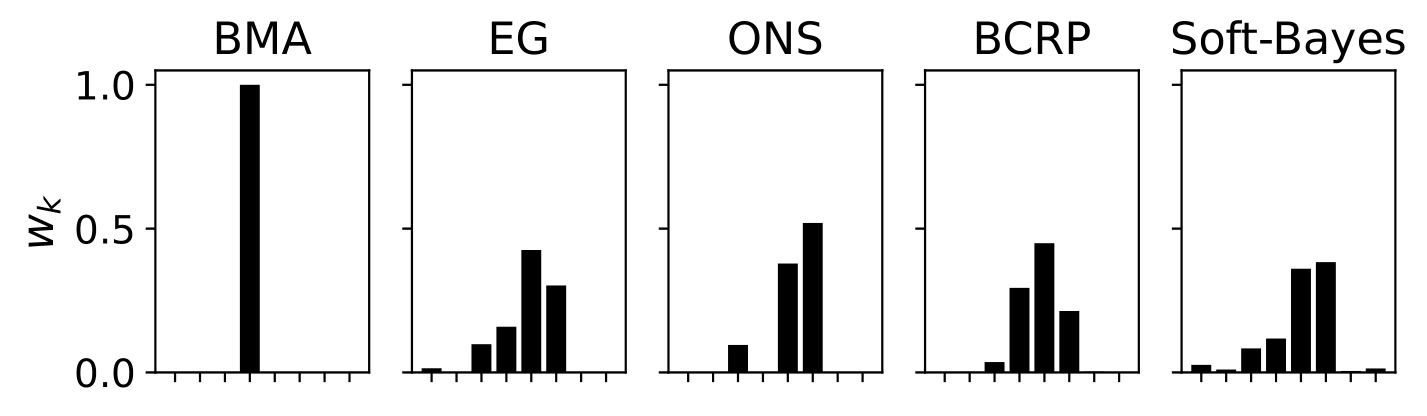
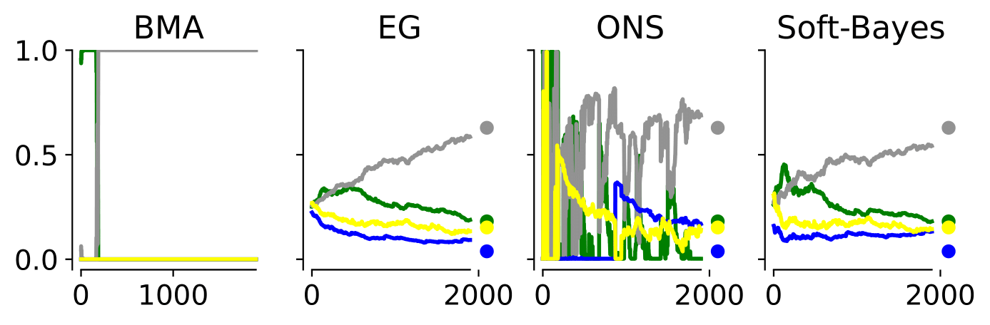
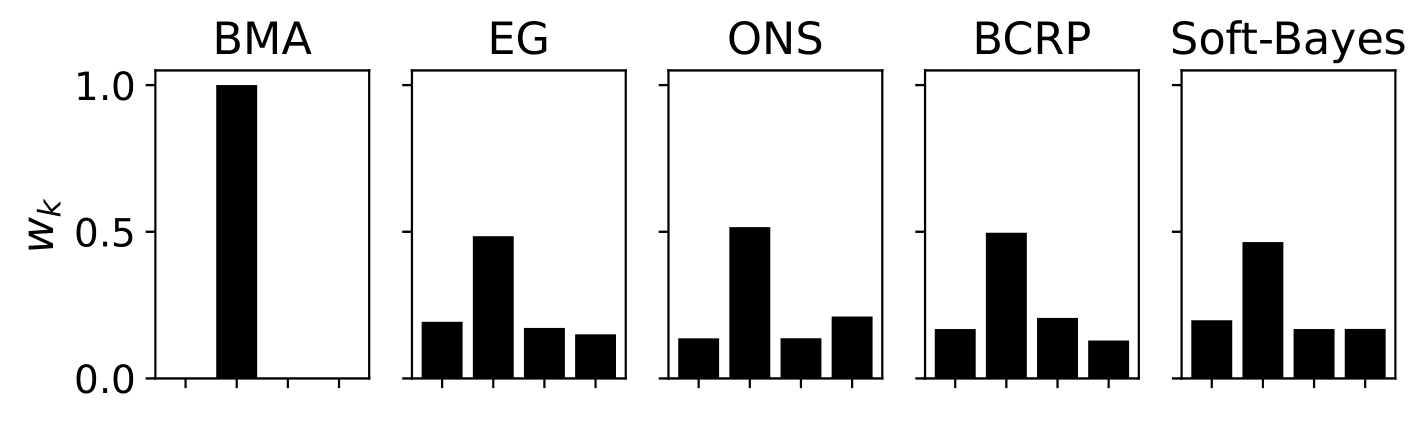
BONG
Application to Filtering
Essentially all of these online Bayesian models amount to some sort of filtering algorithm.
Filtering algorithms use sequential Bayesian inference to update the posterior over some variable \(\theta\) as new data \(y_t\) is observed.
As OBS provides
Indeed, O-BMA is the standard in bank of filter algorithms, e.g., in the GARCH example.
Ongoing Work (Email Me If Interested): OBS can be used to improve classical multiple model filtering, including static multiple model and interacting multiple model filters.
Sequential Learning for Gaussian Processes
Online Ensembles of GPs
Improvements From Filtering
Decentralized Solutions
Learning With Ensembles
OBS was agnostic to how we learned the models in our ensemble -- but how can we train and ensemble simultaneously?
There are two primary challenges here:
- How do we obtain closed-form updates for online learning?
- How do we adapt to non-stationary environments?
These are both difficult to accomplish with GPs in their conventional formulation. We'll address both by reformulating using a linear-Gaussian approximation of GPs.
How Linearization Helps
The point here is that, under a linear-Gaussian approximation to a GP, we can solve for the posterior exactly, via the Kalman filter.
The resulting models are generally known as
To obtain the online ensemble of basis expansions (OEBE), we can additionally combine with OBS or O-BMA.
Random Fourier Features
One popular approximation for stationary GPs are Random Fourier Features (RFF) [Rahimi and Recht, NeurIPS '07].
These features are derived by a Monte Carlo approximation of the Wiener-Khinchin integral
\(\kappa(t, t') = \int_{\mathbb{R}^d} \exp(2\pi i s^\top (t - t')) \, dS(s),\)
where \(S(s)\) is a spectral density and \(i\) is the imaginary unit.
The resulting basis expansion is given by sampling \(F / 2\) spectral frequencies, \(s_1, \dots, s_{F/2}\), and computing the features
\(\phi(x) = \left[ \cos(2\pi s_1^\top x), \sin(2\pi s_1^\top x) \cdots \cos(2\pi s_{F/2}^\top x), \sin(2\pi s_{F/2}^\top x) \right].\)
Takeaway: The RFF provides an approximation that can be sequentially computed, and has computational cost independent of the data size.
Hilbert Space Gaussian Processes
RFF, while simple, suffers harshly from the curse of dimensionality.
Hilbert Space Gaussian Processes (HSGP) [Solin & Sarkka, S&C '20'] address this by instead deriving a quadrature rule over the Wiener-Khinchin integral.
For scalar GPs on \([-L, L]\), the corresponding basis function is
\( \phi_k(t) = S\left(\frac{k\pi}{2L}\right) \frac{\sin\left((k\pi(t+L) / 2L)\right)}{\sqrt{L}}, \quad k = 1, \dots, F. \)
where \(S(s)\) is a spectral density.
Corresponding approximations in higher dimensions are possible but expensive. We instead pursue additive HSGP approximations, which writes \(f(x) = \sum_{d=1}^D f_d(x_d)\).
Takeaway: There are many different basis expansions; these are also a promising place for ensembles.
But What About Dynamic Problems?
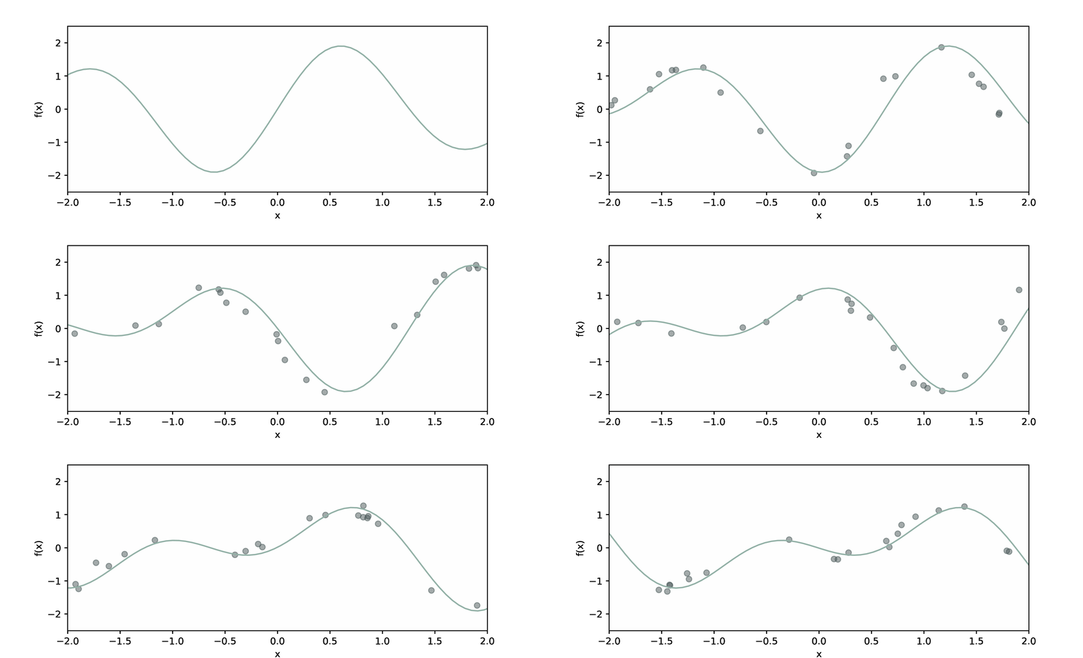
OEBE Fails at Dynamic Problems
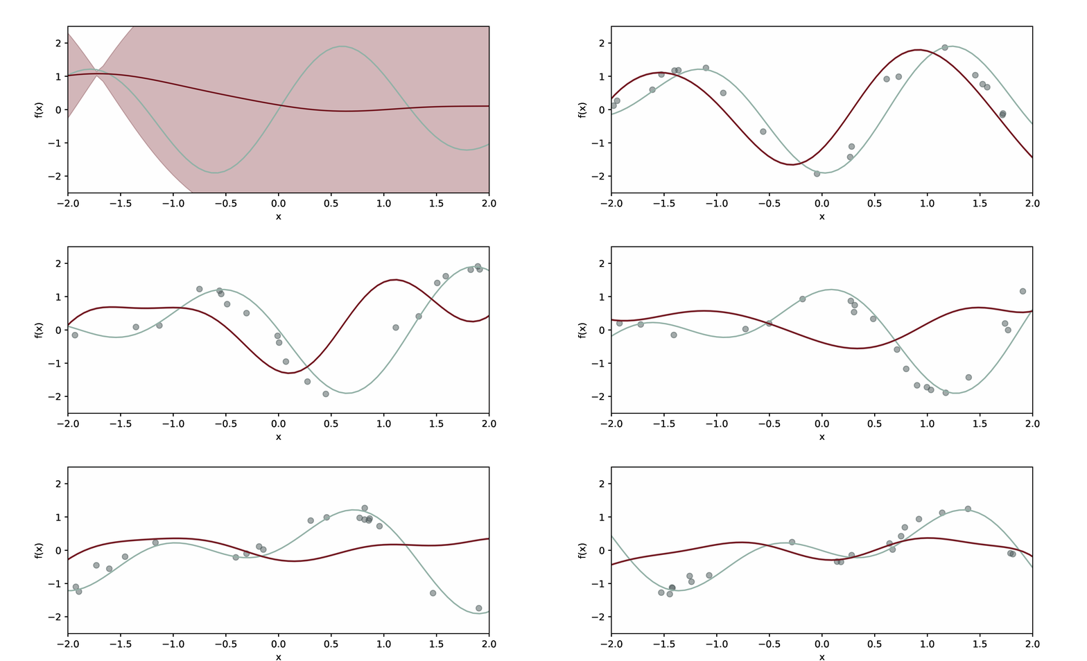
Solution: Parameter Random Walk
From the filtering perspective, a random walk on parameters is an obvious choice.
In particular, with a Gaussian random walk, we maintain exact Kalman filter updates.
We adapt a hyperparameter \(\sigma_\text{rw}^2\), and the state-space model
\( \theta_{t+1}^{(m)} = \theta_t^{(m)} + \varepsilon_{\text{rw}}^{(m)}, \)
and observation model
\( y^{(m)} = \phi^{(m)}(x)^\top \theta_t^{(m)} + \varepsilon_{t}^{(m)}. \)
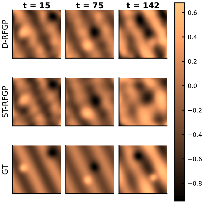
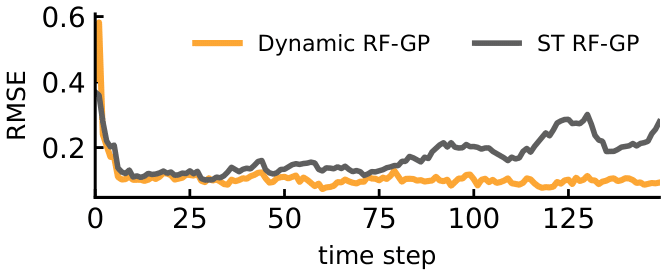
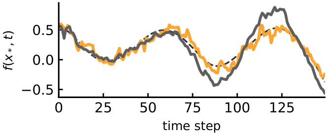
We call the resulting model a distributed online ensemble of basis expansions (DOEBE) [DW & Djuric, TMLR '24].
DOEBE Solves the Dynamic Problems
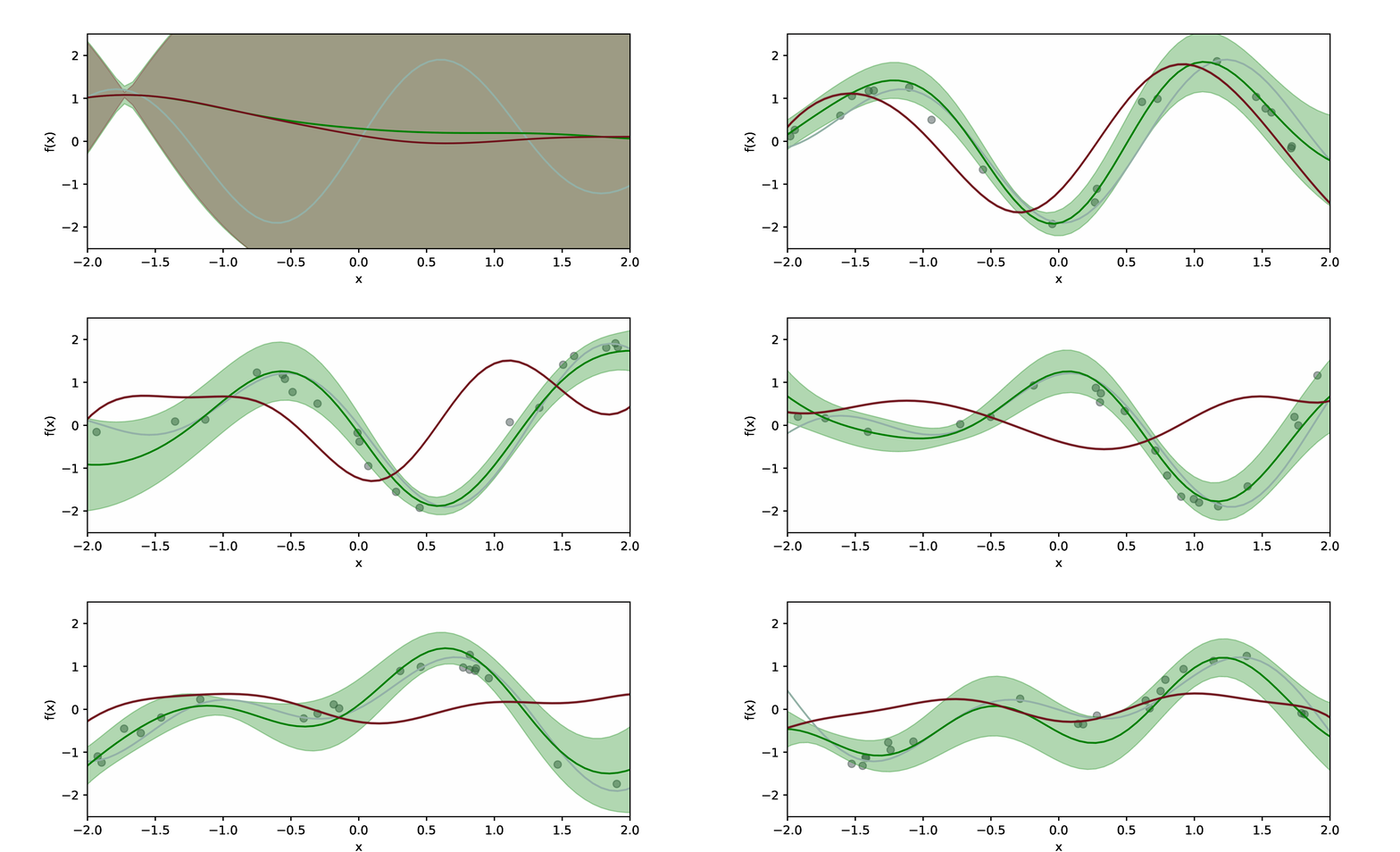
DOEBE Solves the Dynamic Problems
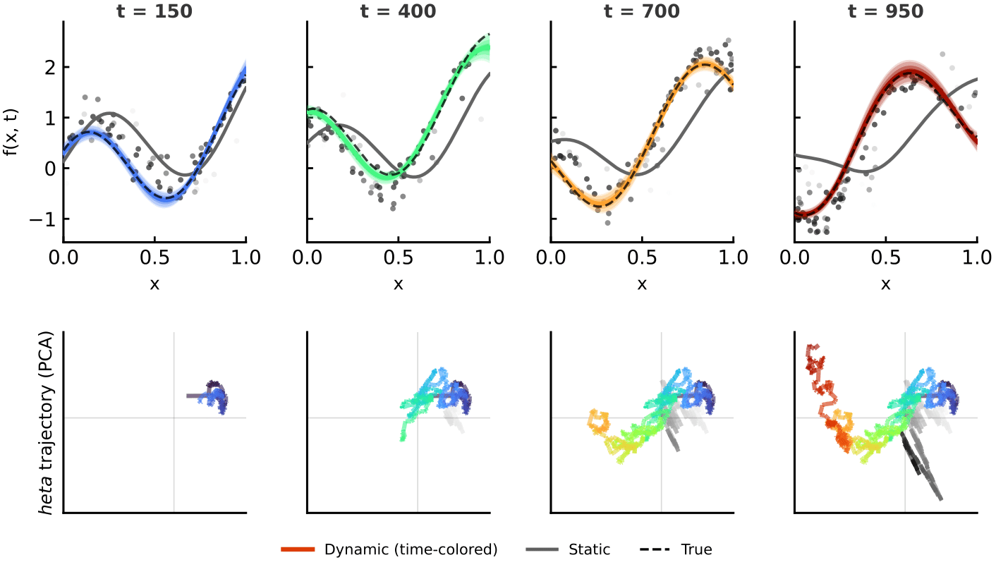
DOEBE Solves the Dynamic Problems
OBS Helps Here Too
Extensions From Filtering Theory
The explicit equivalence with Gaussian filtering opens many opportunities for extensions.
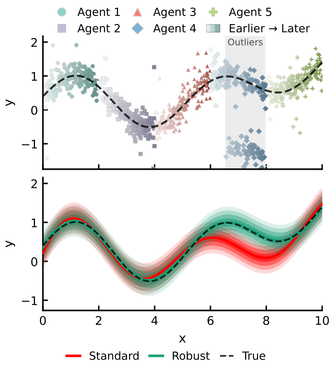
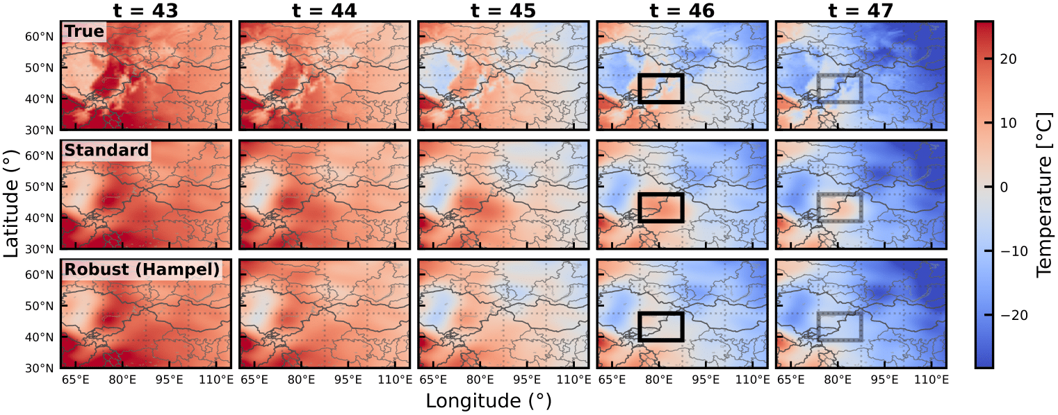
For example, we can use techniques from robust filtering theory for robust GPs.
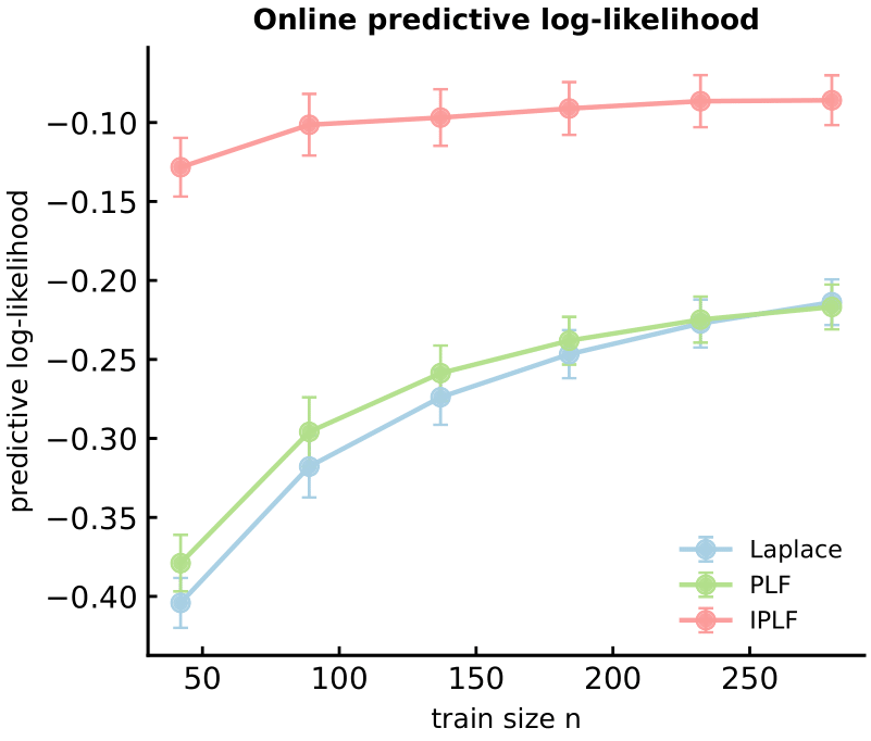
Another example includes stronger non-linear filters through posterior linearization.
Decentralized Solutions
Through similar means, decentralized solutions are possible [Llorente*, DW*, & Djuric, ICASSP '25; Llorente, DW, et al., ICASSP '26].
These fall from using the information form of the Kalman filter, which makes all quantities additive.
Strong consensus algorithms are thus available, and provide decentralized inference that is asymptotically exact.
Dynestyx: A Probabilistic Programming Language for Dynamical Systems
Ongoing Work with Matt Levine
Dynestyx: A Probabilistic Programming Language for Dynamical Systems
Our solutions to online inference have worked by translating to the language of dynamical systems.
This is quite powerful, for a few reasons:
- The resulting problem is naturally sequential, which is already close to online inference.
- The problem is well-studied, with many bespoke algorithms and approximations.
But how can non-experts exploit these powerful solutions easily?

def continuous_time_lingam_model():
				"""2D linear SDE with a sampled coupling."""
				rho = numpyro.sample("rho", dist.Uniform(0.0, 5.0))

				A = jnp.array([[-1.0, 0.0], [rho, -1.0]])

				dynamics = DynamicalModel(
					state_dim=2,
					observation_dim=1,
					initial_condition=dist.MultivariateNormal(
						loc=jnp.zeros(2), covariance_matrix=1.0**2 * jnp.eye(2)
					),
					state_evolution=ContinuousTimeStateEvolution(
						drift=lambda x, u, t: A @ x,
						diffusion_coefficient=lambda x, u, t: jnp.eye(2),
						diffusion_covariance=lambda x, u, t: jnp.eye(2),
					),
					observation_model=LinearGaussianObservation(
						H=jnp.array([[0.0, 1.0]]), R=jnp.array([[1.0**2]])
					),
				)
				return sample_ds("f", dynamics)
observation_trajectory = Trajectory(times=obs_times, values=obs_values)

def data_conditioned_model():
    context = Context(observations=observation_trajectory)
    with FilterBasedMarginalLogLikelihood(
    	filter_type="dpf", dpf_num_particles=2_500)
    ):
        with Condition(context):
            return continuous_time_lingam_model()


mcmc_key = jr.PRNGKey(0)
nuts_kernel = NUTS(data_conditioned_model)
mcmc = MCMC(nuts_kernel, num_samples=num_samples, num_warmup=num_samples)
mcmc.run(mcmc_key)
observation_trajectory = Trajectory(times=obs_times, values=obs_values)
def data_conditioned_model():
context = Context(observations=observation_trajectory)
with FilterBasedMarginalLogLikelihood(
filter_type="dpf", dpf_num_particles=2_500)
):
with Condition(context):
return continuous_time_lingam_model()
mcmc_key = jr.PRNGKey(0)
nuts_kernel = NUTS(data_conditioned_model)
mcmc = MCMC(nuts_kernel, num_samples=num_samples, num_warmup=num_samples)
mcmc.run(mcmc_key)observation_trajectory = Trajectory(times=obs_times, values=obs_values)
def data_conditioned_model():
context = Context(observations=observation_trajectory)
with FilterBasedMarginalLogLikelihood(
filter_type="enkf", enkf_num_particles=100)
):
with Condition(context):
return continuous_time_lingam_model()
mcmc_key = jr.PRNGKey(0)
nuts_kernel = NUTS(data_conditioned_model)
mcmc = MCMC(nuts_kernel, num_samples=num_samples, num_warmup=num_samples)
mcmc.run(mcmc_key)Example: Defining the Online RFF GP
def rff_features(x, omegas, phases):
    x = jnp.asarray(x)
    x = jnp.squeeze(x)
    return jnp.sqrt(2.0 / omegas.shape[0]) * jnp.cos(omegas * x + phases)

class RFFInputObservation(ObservationModel):
    omegas: jax.Array
    phases: jax.Array
    sigma_y: float

    def __call__(self, x, u, t):
        phi_x = rff_features(u, self.omegas, self.phases)
        mean = jnp.dot(phi_x, x)
        return dist.Normal(loc=mean, scale=self.sigma_y)
Example: Defining the Online RFF GP
def dynamic_rff_gp_numpyro_model(omegas, phases, sigma_y, sigma_rw):
    state_dim = omegas.shape[0]
    initial_condition = dist.MultivariateNormal(
        loc=jnp.zeros(state_dim), covariance_matrix=jnp.eye(state_dim)
    )

    dynamics = DynamicalModel(
        state_dim=state_dim,
        observation_dim=1,
        control_dim=1,
        initial_condition=initial_condition,
        state_evolution=GaussianRandomWalk(state_dim, sigma_rw),
        observation_model=RFFInputObservation(
            omegas=omegas, phases=phases, sigma_y=sigma_y
        ),
        continuous_time=False,
    )

    return dsx.sample("f", dynamics)
Example: Defining the Online RFF GP
def data_conditioned_model():
    observation_trajectory = Trajectory(times=obs_times, values=obs_values)
    context = Context(
        observations=observation_trajectory,
        controls=Trajectory(times=obs_times, values=x_controls),
    )
    with FilterBasedMarginalLogLikelihood(
        filter_type="taylor_kf",
        record_filtered_states_mean=True,
        record_filtered_states_cov=True,
    ):
        with Condition(context=context):
            return dynamic_rff_gp_numpyro_model(omegas, phases, sigma_y, sigma_rw)

filter_predictive = Predictive(
	data_conditioned_model,
    num_samples=1,
    exclude_deterministic=False
)
filter_outputs = filter_predictive(jr.PRNGKey(1))
Future Directions
Dynestyx gives a way to rapidly prototype for applications: let's find those applications!
With applications in-hand, understand how estimation methods actually fail, in practice, and when.
With our programmatic tools, learn how to do proper hybrid modeling, i.e., when we mix mechanistic understanding with data-driven components.
Summary
Summary
As ML methods become more complex and capable, online and scalable inference remain challenging.
Sequential Bayesian inference provides a principled framework to accomplish such requirements.
Using recent developments in Bayesian ML, online convex optimization, and scientific computing, we propose scalable solutions to online ensembles, all using sequential Bayes as a core principle.
We also introduce dynestyx, a probabilistic programming language for dynamical systems, which allows non-experts to use state-of-the-art sequential Bayes for their own problems.
Questions?
Contact: dan@basis.ai
References:
[1] DW, Llorente, & Djurić (2026). Bayesian Ensembling: Insights from Online Optimization and Empirical Bayes. Transactions on Machine Learning Research.
[2] DW & Djurić (2024). Dynamic online ensembles of basis expansions. Transactions on Machine Learning Research.
[3] Llorente*, DW*, & Djurić (2025). Decentralized Online Ensembles of Gaussian Processes for Multi-Agent Systems. ICASSP 2025.
[4] Llorente, DW, & Djurić (2026). Robust, Online, and Adaptive Decentralized Gaussian Processes. ICASSP 2026.