A Bayesian Recipe for Learning
Hybrid Models from Noisy Data.
Joint/ongoing work with Matt Levine, Matthieu Darcy, Youssef Marzouk, and others.

SIAM NE 2026 Meeting
August 22, 2026
Hybrid Models
Many modern tasks consist of prior, mechanistic knowledge that we want to use and hold on to, but we know is incomplete.
Among other things, it motivates the framework of universal differential equations [Rackauckas et al., 2020].
A hybrid model is the statistical realization of this pattern, combining a known and unknown mechanism.
For example, in continuous time:
\(\def\V#1{\boldsymbol{\mathbf{#1}}} \mathrm{d}\V{x}_t = \left(f_{\mathrm{known}}(\V{x}_t) + f_{\mathrm{unknown}}^{\V\theta}(\V{x}_t)\right)\mathrm{d}t + \left(g_{\mathrm{known}}(\V{x}_t) + g_{\mathrm{unknown}}^{\V\theta}(\V{x}_t)\right)\mathrm{d}\V\beta_t.\)
Implementation Is the Hard Part
Writing down a hybrid model is easy. Making it behave is not:
- How do I write \(f_{\mathrm{unknown}}\) so that it does not overpower my prior knowledge \(f_{\mathrm{known}}\)?
- How do I set priors on such a thing?
- How do I do proper uncertainty quantification?
The solution I present is not fancy — from a Bayesian perspective it is the straightforward "right" thing to do.
The point is to show how it may work, and that it deals naturally with things like UQ, partial observations, noisy observations, and arbitrary missingness patterns.
Three Goals
Goal 1. Show a simple Bayesian recipe for hybrid dynamical systems: that it can work, and that you may want to use it.
Goal 2. Show how dynestyx
[DW et al., 2026] makes this modeling explicit, efficient,
and easy to use.
Goal 3. Convince you that you should work on these :).
dynestyx
Bayesian State-Space Models
dynestyx is a probabilistic programming library with first-class support for
state-space models, on a JAX backend [DW et al., 2026].
A latent state \(\def\V#1{\boldsymbol{\mathbf{#1}}}\V{x}(t) \in \mathbb{R}^{d_x}\) evolves in continuous time,
\(\def\V#1{\boldsymbol{\mathbf{#1}}}\mathrm{d}\V{x}(t) = f_{\V\theta}(\V{x}(t), t)\,\mathrm{d}t + g_{\V\theta}(\V{x}(t), t)\,\mathrm{d}\V\beta_t,\)
or in discrete time, \(\def\V#1{\boldsymbol{\mathbf{#1}}}\V{x}_t \sim p_{\V\theta}(\V{x}_t \mid \V{x}_{t-1})\). Observations arrive at discrete times as \(\def\V#1{\boldsymbol{\mathbf{#1}}}\V{y}_t \sim p_{\V\phi}(\V{y}_t \mid \V{x}_t)\).
State estimation asks for posteriors over the state: filtering \(\def\V#1{\boldsymbol{\mathbf{#1}}}p(\V{x}_t \mid \V{y}_{1:t})\), smoothing, and forecasting.
System identification asks for posteriors over parameters,
\(\def\V#1{\boldsymbol{\mathbf{#1}}}p(\V\theta, \V\phi \mid \V{y}_{1:T}) \propto p(\V\theta, \V\phi)\,p(\V{y}_{1:T} \mid \V\theta, \V\phi).\)
dynestyx
A Unified Interface
Model specification is general and simple. For example, to write an arbitrary drift, unit diffusion, and a Poisson observation model.
def model(obs_times, obs_values, ctrl_times, ctrl_values, predict_times):
    theta = numpyro.sample("theta", p_theta)

    continuous_state_evolution = ContinuousTimeStateEvolution(
        drift=f_drift(theta),
        # More efficient, but arbitrary JAX functions are allowed
        diffusion=ScalarDiffusion(0.1),
    )

    dynamics = DynamicalModel(
        initial_condition=dist.Normal(0, 1),
        state_evolution=continuous_state_evolution,  # or discrete time!
        observation_model=dist.Poisson(...),
    )

    return dsx.sample("f", dynamics,
                      obs_times=obs_times, obs_values=obs_values,
                      predict_times=predict_times)
Data enters through obs_times and obs_values; predictions come
out at predict_times.
dynestyx
Separation of Concerns
State-space models are full of approximations: how the state is marginalized, how time is discretized, how parameters are inferred. Semnatically, this isn't the model's job.
Filtering and smoothing are inference choices,
not model choices. So dsx.sample is an effectful operation,
interpreted at inference time by whichever handler is in scope.
with Filter(EKFConfig()):
    filtered = predictive_model(obs_times=obs_times, obs_values=obs_values)

with Filter(EnKFConfig(n_particles=50)):
    filtered = predictive_model(obs_times=obs_times, obs_values=obs_values)

with Smoother():
    smoothed = predictive_model(obs_times=obs_times, obs_values=obs_values)
The model code never changes.
dynestyx
Mix 'n' Match
Any filter, smoother, or simulator composes with any NumPyro inference algorithm.
with Filter(filter_config):
    with Discretizer(ODEFlowConfig(...)):
        mcmc = MCMC(NUTS(model), ...)
        mcmc.run(...)
        # or
        svi = SVI(model, AutoNormal(model), ...)
        svi.run(...)
Some mildly novel combinations turn out to work well: MALA with a particle filter, NUTS with an EnKF, and — the one we use today — SVI with an EnKF.
We also support hierarchical inference, closed-loop control, and lots more!
The Bayesian Recipe
Five Steps
Sparse Dictionaries
HSGP Closures
DW, Batenkov, D., Feser, J., Zane, A., Bingham, E., Marzouk, Y., & Levine, M. (2026). Dynestyx: A Probabilistic Programming Library for Dynamical Systems. arXiv:2606.16985.
The Recipe
We break our recipe into five steps:
- Write down the known mechanistic component \(f_{\mathrm{known}}, g_{\mathrm{known}}\), and any priors it carries.
- Put a prior on the unknown components \(f_{\mathrm{unknown}}^{\theta}\) and, where needed, \(g_{\mathrm{unknown}}^{\theta}\).
- Specify the observation likelihood \(\def\V#1{\boldsymbol{\mathbf{#1}}}p(\V{y}_t \mid \V{x}_t, \V\theta)\) and priors for unknown observation parameters.
- Choose a method for marginalizing the dynamical system. We use an EnKF, which we find very effective; others are certainly possible.
- Choose a method for inference on \(\def\V#1{\boldsymbol{\mathbf{#1}}}\V\theta\). We use black-box stochastic variational inference.
This is really one part of a larger Bayesian workflow; today we focus on model building.
Priors Over Unknown Components
We use two generic families throughout.
Sparse dictionary. A small set of low-degree polynomial terms with a Laplace prior to shrink coefficients — analogous to SINDy [Brunton et al., 2016]. When it works, results are interpretable and data-efficient... it does not always work.
HSGP closure. A Gaussian process prior on \(f_{\mathrm{unknown}}\); we'll use a squared-exponential kernel, treated fully Bayesian.
To make this tractable we use the Hilbert space GP approximation [Solin & Särkkä, 2020] — a truncated Karhunen–Loève-like expansion on a bounded domain with Dirichlet boundary conditions. What matters here is that we end up with
\(\def\V#1{\boldsymbol{\mathbf{#1}}}f(\V{x}_t) \approx \V\theta^\top \V\phi(\V{x}_t; \ell, \sigma).\)
An ODE Example: Multiscale Lorenz–96
The Reduced Model
Four Bayesian Models
Missing Observations
Multiscale Lorenz–96
The two-scale Lorenz–96 system has \(K = 9\) slow variables, with \(J = 8\) fast variables attached to each slow coordinate:
\[\begin{aligned} \dot X_k &= -X_{k-1}(X_{k-2} - X_{k+1}) - X_k + F + h_x \bar Z_k, \\ \dot Z_{k,j} &= \frac{-Z_{k,j+1}(Z_{k,j+2} - Z_{k,j-1}) - Z_{k,j} + h_y X_k}{\varepsilon}, \qquad \bar Z_k = \frac{1}{J}\sum_{j=1}^J Z_{k,j}, \end{aligned}\]
with circular indexing and
\(\varepsilon = 2^{-5}, \qquad h_x = -0.8, \qquad h_y = 1, \qquad F_\star = 10.\)
The model is chosen so that a Markovian closure is possible [Levine & Stuart, 2022].
The Reduced Model
To specify a reduced model, we simply omit all observation and knowledge of the fast states. Naïvely, this leaves
\(\dot X_k = -X_{k-1}(X_{k-2} - X_{k+1}) - X_k + F + c(X_k).\)
We simulate from the full system with \(4.0\) time units of burn-in, \(10.0\) of training data, and \(4.0\) of test rollout. Observations arrive every \(0.1\) time units.
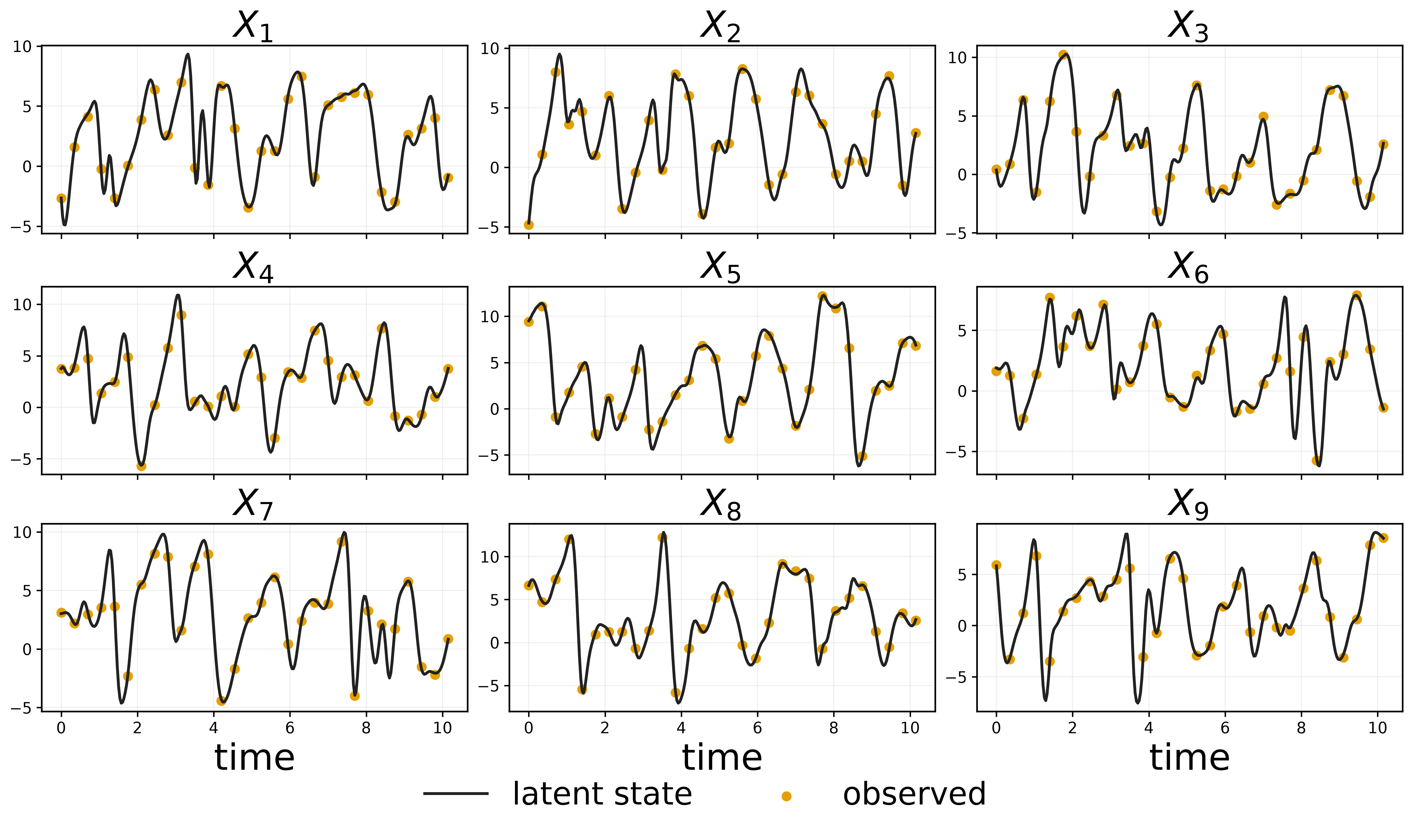
The baseline noisily observes every resolved coordinate \(X_1, \ldots, X_9\) with independent Gaussian noise of standard deviation \(\sigma_{y,\star} = 0.15\). All \(72\) fast coordinates remain hidden.
Training Data
The nine slow coordinates, and what the reduced model actually gets to see.
Inference Targets
We leave the forcing \(F\) and the observation scale \(\sigma_y\) unknown, with priors
\(F \sim \mathcal{N}(10.0, 2.0^2), \qquad \sigma_y \sim \operatorname{HalfNormal}(0.25).\)
Recovering these interpretable quantities is a primary scientific target.
We also want to learn the closure \(c\), which is what lets us do state estimation. So we measure three things:
- parameter recovery,
- filtered-state accuracy, and
- held-out forecast accuracy.
Four Bayesian Reduced Models
Naïve Bayes. The fully-reduced model, \(c(x) = 0\).
SDE Relaxation. Model the missing components generically, as a stochastic term:
\(\mathrm{d}X_k = \left[-X_{k-1}(X_{k-2} - X_{k+1}) - X_k + F\right]\mathrm{d}t + q\,\mathrm{d}W_t.\)
Sparse closure. A dictionary in the rescaled state (\(x_k\) divided by \(10\)):
\(c_{\mathrm{sparse}}(x_k) = \beta_1 x_k + \beta_2 x_k^2 + \beta_3 x_k^3, \qquad \beta_j \sim \operatorname{Laplace}(0, 0.5).\)
HSGP closure. Ten squared-exponential basis modes on the scaled domain \([-1.5, 1.5]\), standard-normal basis weights, a half-normal prior on kernel variance, and a log-normal prior on length scale.
An unrestricted intercept in \(c\) would confound \(F\). We rule it out by construction: the dictionary has \(c(0) = 0\), and the HSGP subtracts off \(f(0)\).
Writing This Down in dynestyx
The base model: no closure at all
def slow_l96_drift(x, forcing):
    return -jnp.roll(x, 1) * (jnp.roll(x, 2) - jnp.roll(x, -1)) - x + forcing

def model(obs_times=None, obs_values=None, predict_times=None):
    forcing = numpyro.sample("F", dist.Normal(10.0, 2.0))
    obs_sigma = numpyro.sample("obs_sigma", dist.HalfNormal(0.25))

    def drift(x, u, t):
        return slow_l96_drift(x, forcing)

    dynamics = DynamicalModel(
        initial_condition=dist.MultivariateNormal(mu_0, covariance_matrix=Sigma_0),
        state_evolution=ContinuousTimeStateEvolution(drift=drift),
        observation_model=LinearGaussianObservation(
            H=H_OBS, R=obs_sigma**2 * jnp.eye(len(OBSERVED_INDICES))
        ),
    )
    return dsx.sample(
        "f", dynamics, obs_times=obs_times, obs_values=obs_values,
        predict_times=predict_times
    )
Writing This Down in dynestyx
The sparse closure: three new lines
def slow_l96_drift(x, forcing):
    return -jnp.roll(x, 1) * (jnp.roll(x, 2) - jnp.roll(x, -1)) - x + forcing

def model(obs_times=None, obs_values=None, predict_times=None):
    forcing = numpyro.sample("F", dist.Normal(10.0, 2.0))
    obs_sigma = numpyro.sample("obs_sigma", dist.HalfNormal(0.25))
    beta = numpyro.sample(
        "beta", dist.Laplace(0.0, 0.5).expand([3]).to_event(1)
    )

    def drift(x, u, t):
        return slow_l96_drift(x, forcing) + dictionary(x / 10.0, beta)

    dynamics = DynamicalModel(
        initial_condition=dist.MultivariateNormal(mu_0, covariance_matrix=Sigma_0),
        state_evolution=ContinuousTimeStateEvolution(drift=drift),
        observation_model=LinearGaussianObservation(
            H=H_OBS, R=obs_sigma**2 * jnp.eye(len(OBSERVED_INDICES))
        ),
    )
    return dsx.sample(
        "f", dynamics, obs_times=obs_times, obs_values=obs_values,
        predict_times=predict_times
    )
Approximate Inference
We discretize the ODE and use an ensemble Kalman filter to marginalize the states, then SVI with clipped Adam and one Monte Carlo particle per ELBO estimate [Tran et al., 2017].
Both are interpretations wrapped around the same model code — and missing
observations need no model change at all. We mark them with NaN.
with Filter(filter_config=EnKFConfig(...)):
    with Discretizer(ODEFlowConfig(...)):
        guide = AutoMultivariateNormal(
            reduced_model, init_loc_fn=init_to_mean(), init_scale=0.08
        )
        svi = SVI(
            reduced_model, guide,
            numpyro.optim.ClippedAdam(step_size=3e-3, clip_norm=10.0),
            loss=Trace_ELBO(num_particles=1),
        )
        result = svi.run(
            key, num_steps=num_steps,
            obs_times=obs_times, obs_values=training_obs_values,
        )
Recovering the Forcing
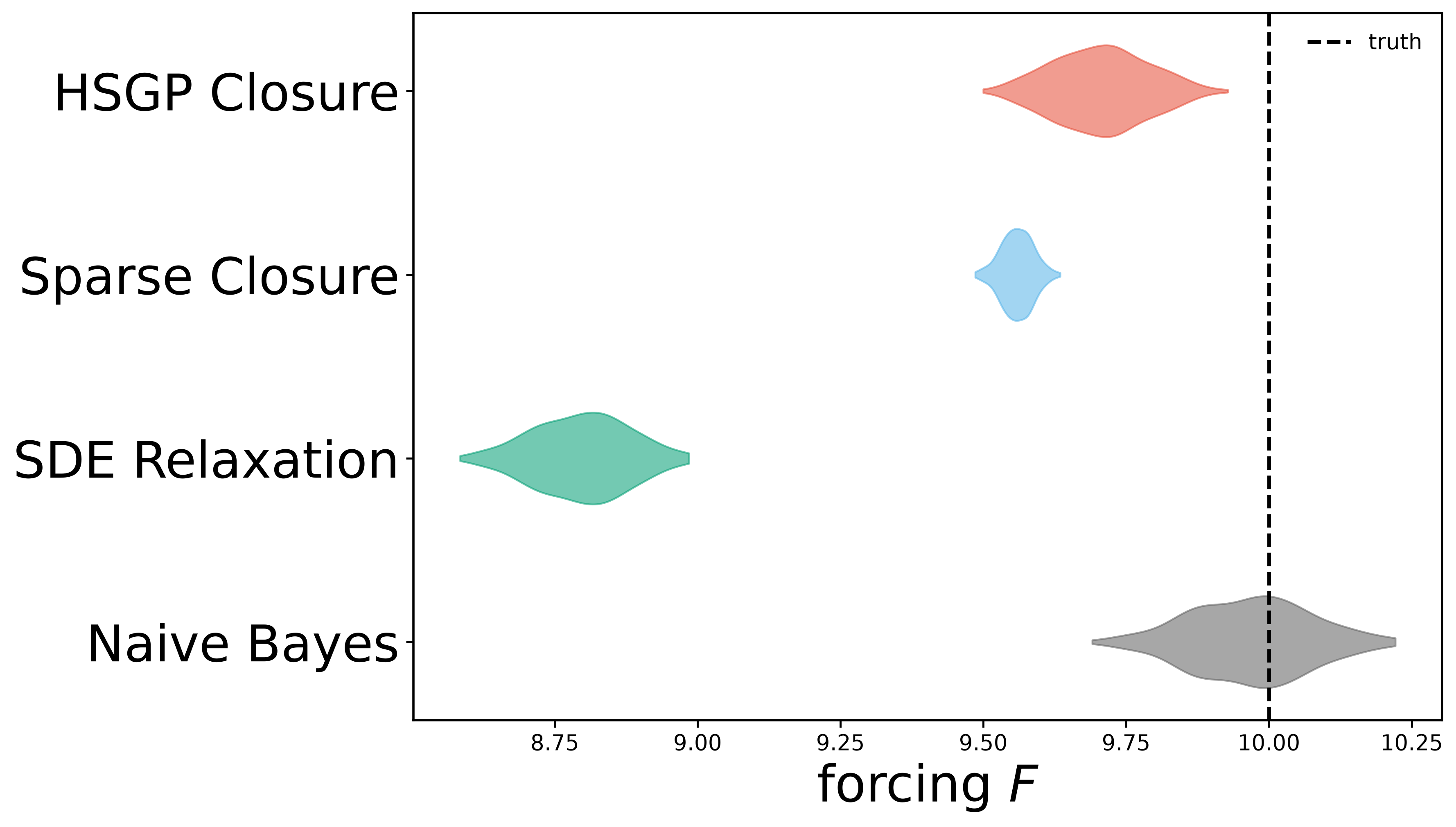
One benefit of a closure is that we retain good inference and UQ on the interpretable parameters.
In the ODE case, \(F\) is statistically learnable even without a closure: if \(\bar Z\) is zero-mean, it simply averages out. The SDE relaxation, on the other hand, corrupts it.
The Learned Closure
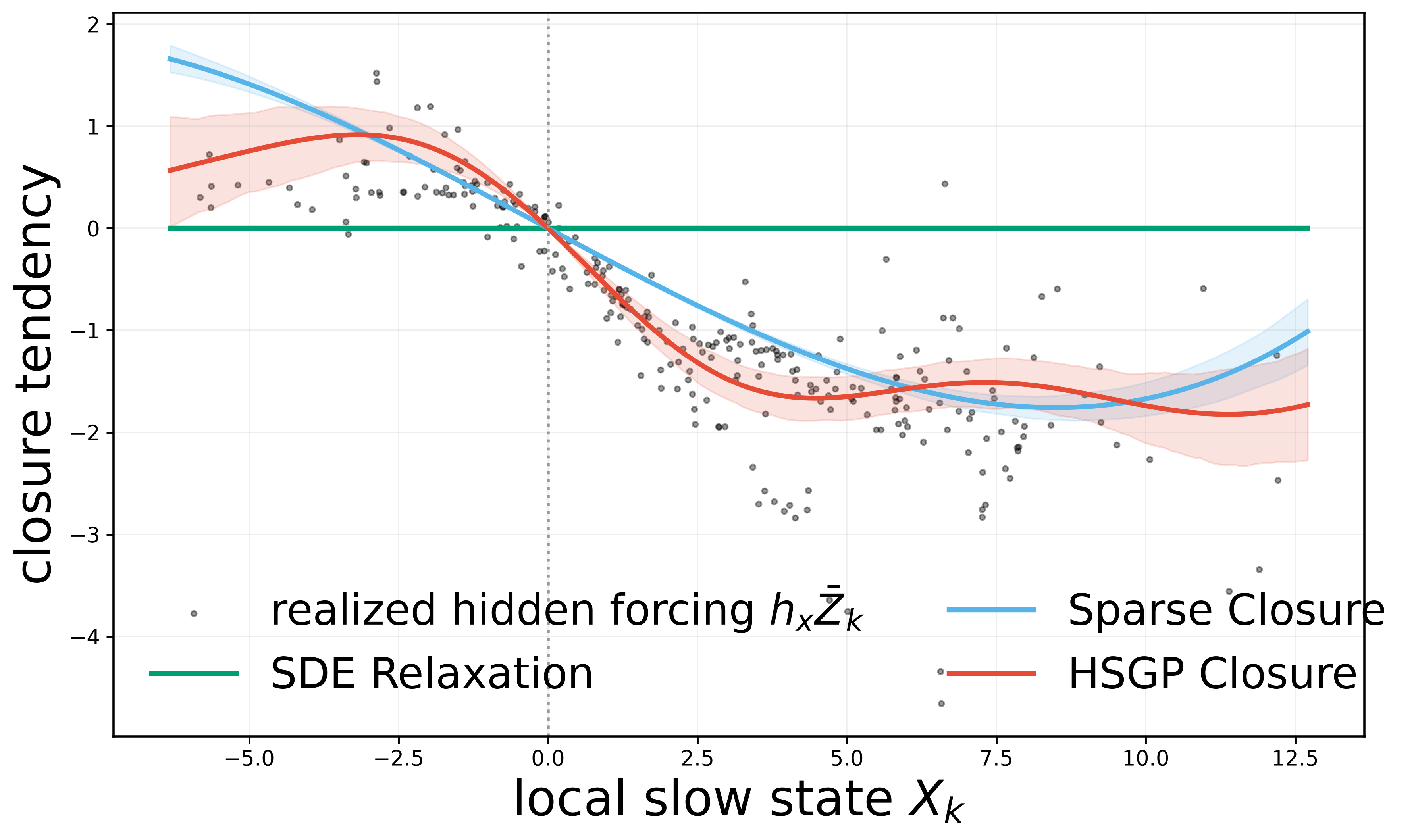
Both hybrid models recover the sign and shape of the hidden forcing \(h_x \bar Z_k\), with some amount of uncertainty.
Filtering
So what is the drawback of the mis-specified model?
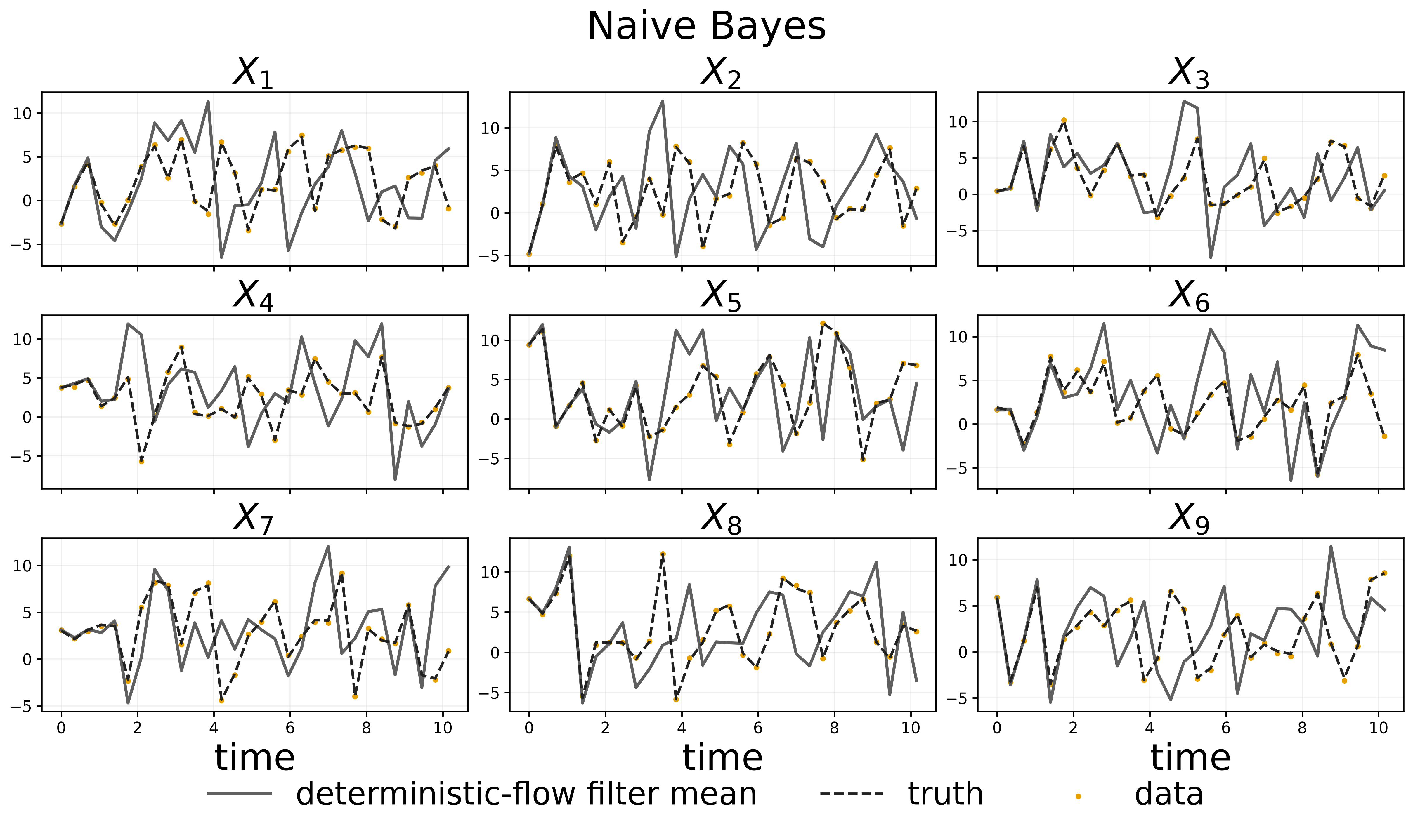
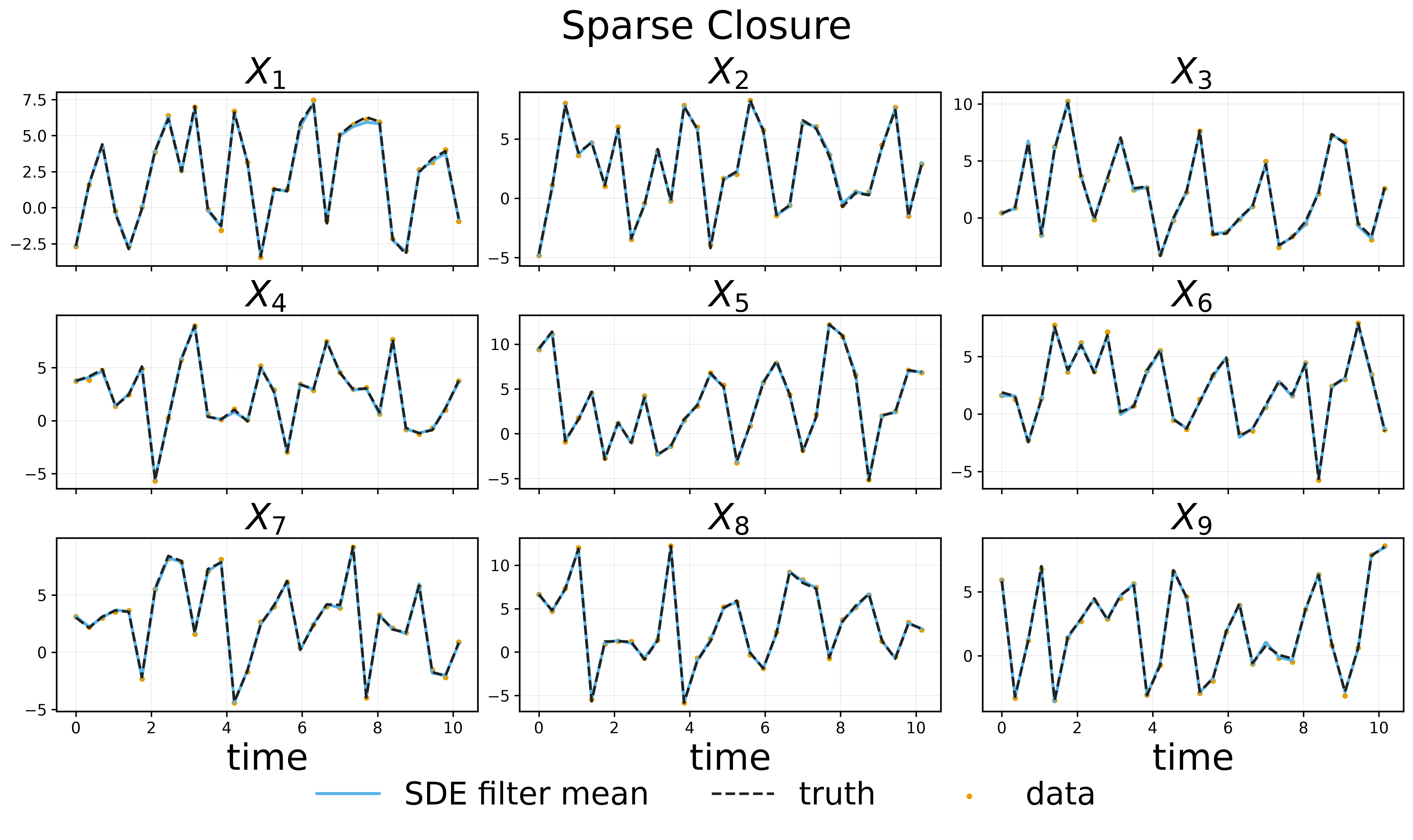
The SDE relaxation filters well too, but by inflating stochastic noise to compensate.
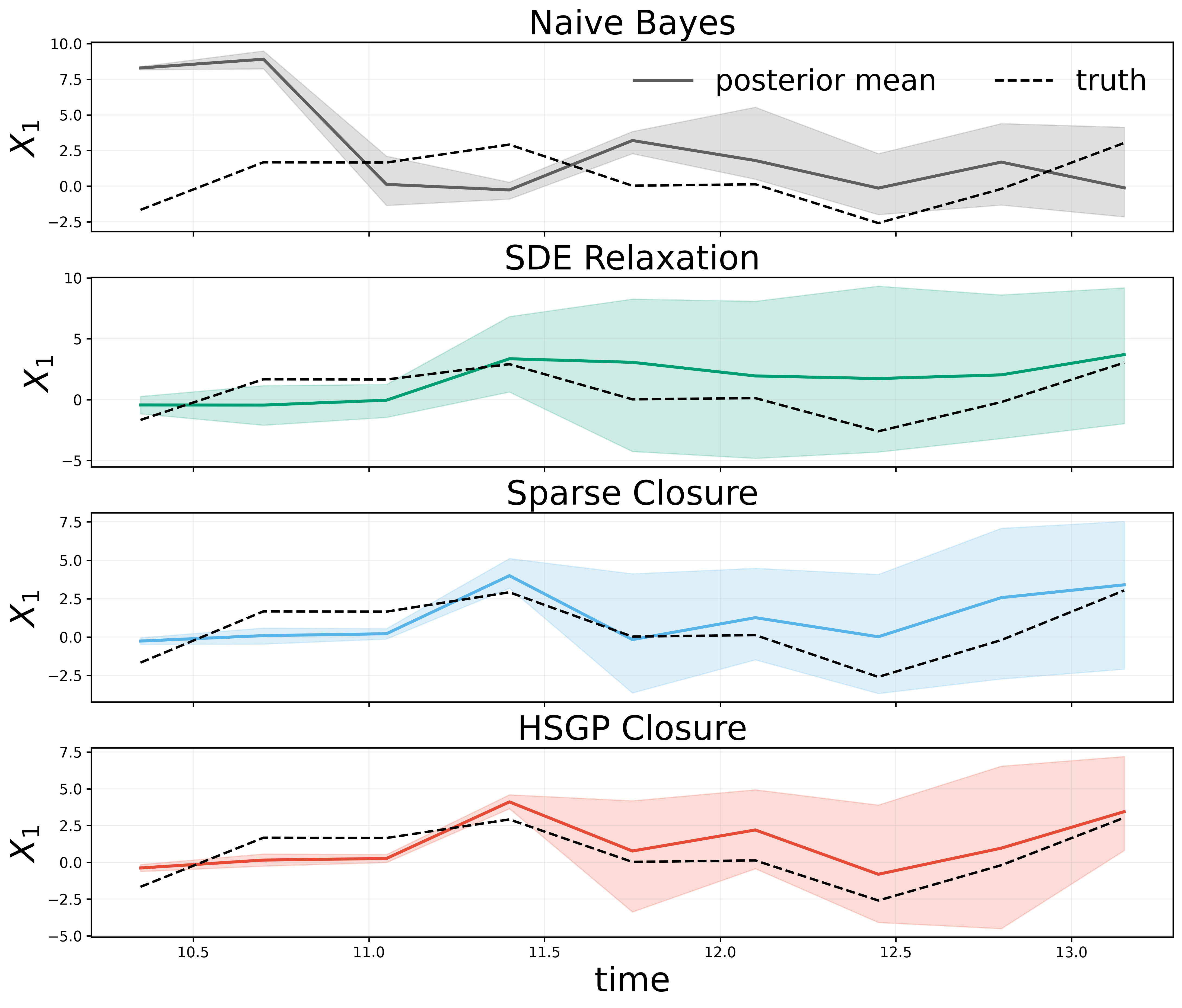
Forecasting
The SDE relaxation and naive ODE method are also both poor at forecasting.
Missing Observations
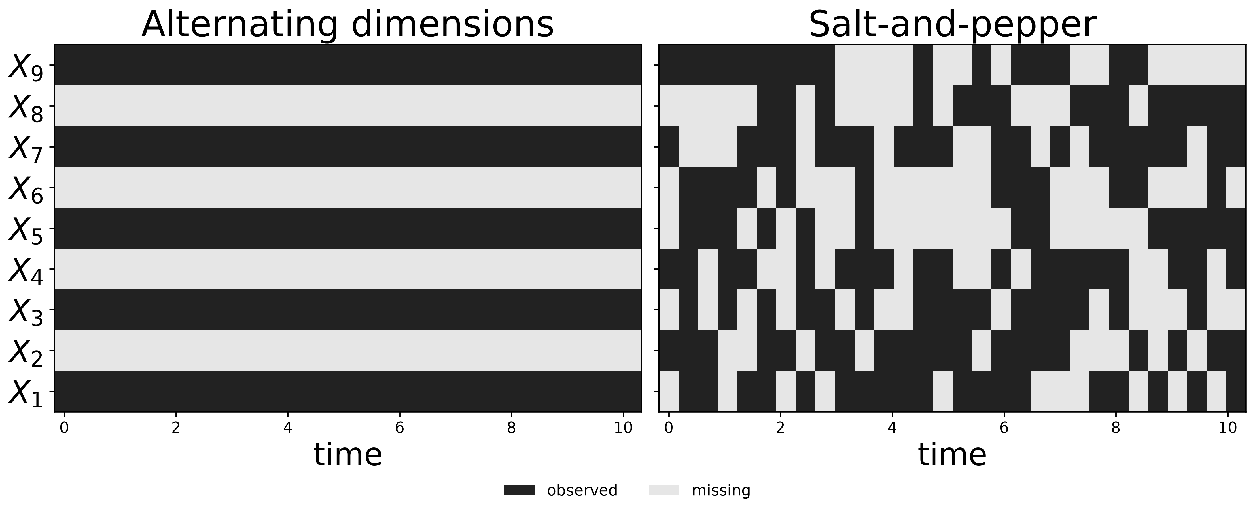
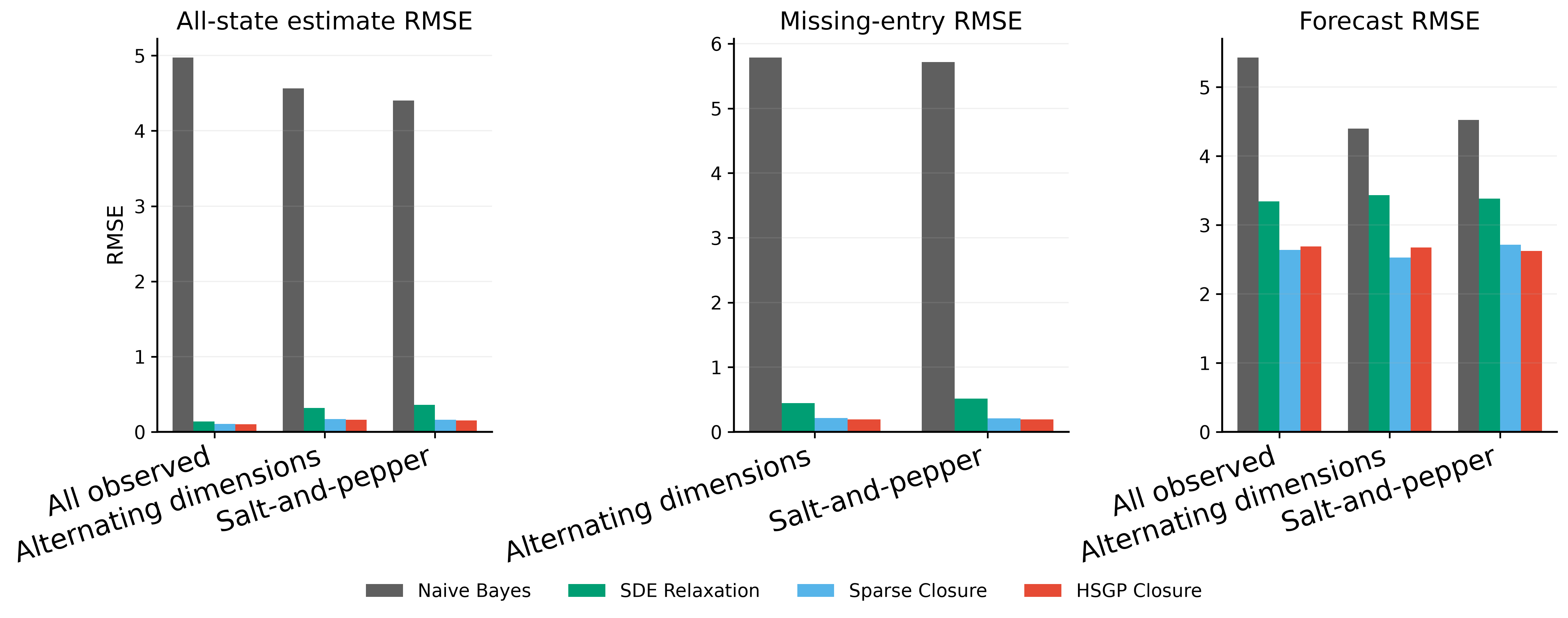
Alternating dimensions. We always observe \(X_1, X_3, X_5, X_7, X_9\) (and never \(X_2, X_4, X_6, X_8\)). i.e., the states and closure must be recoverable from a subset of components.
Salt-and-pepper. We randomly drop ~55% of observations, across time and component.
Neither our methods nor dynestyx care much either way; each
model is refit by exactly the same recipe (and code!).
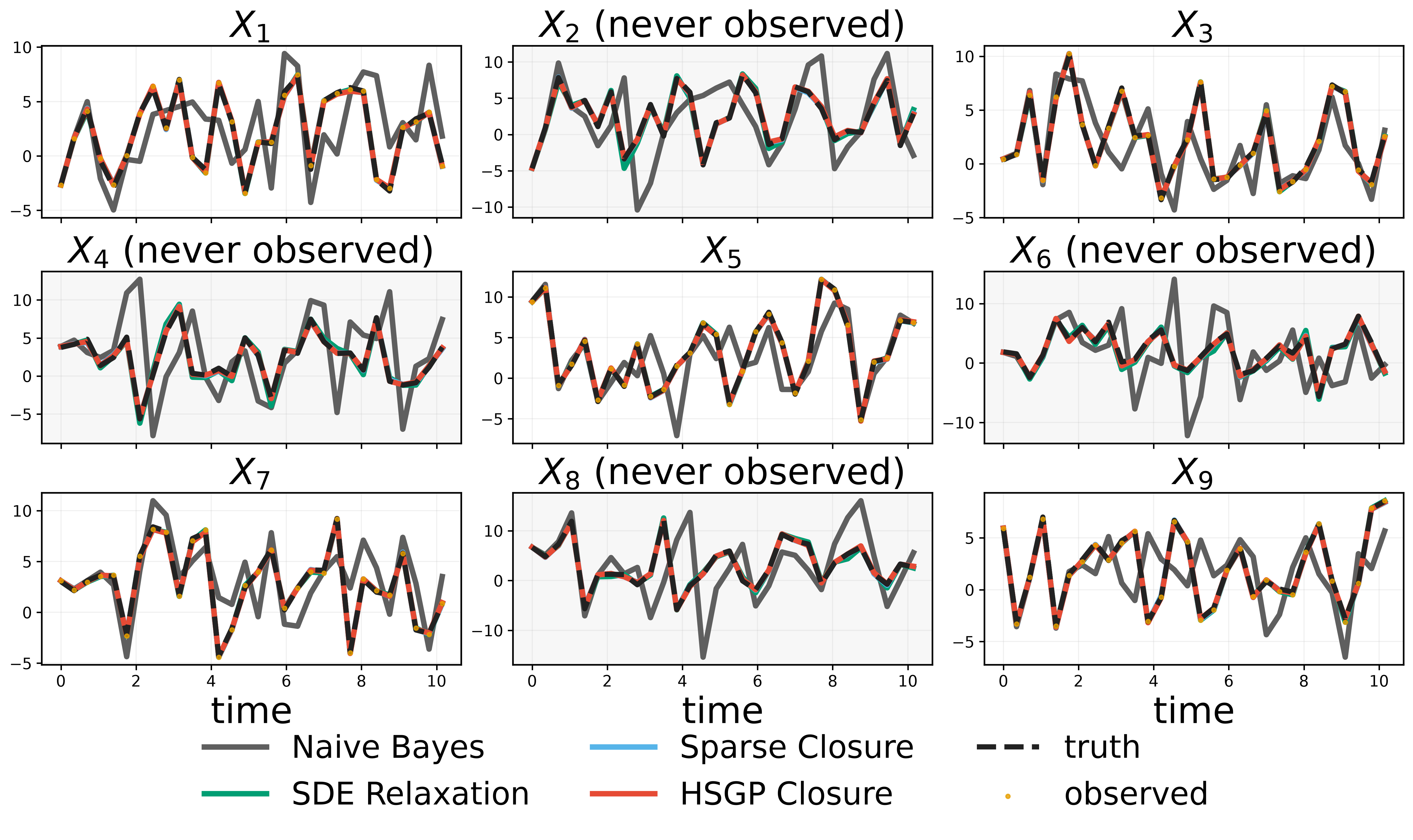
Reconstructing Never-Observed Coordinates
The hybrid models (and SDE relaxation) are able to perform this task well; the naive model doesn't.
Performance Under Missingness
Closure models outperform the baselines, even under missingness, while maintaining meaningfull parameters.
A PDE Example: The Fisher–KPP Reaction
The Method of Lines
Learning the Reaction
Filtering vs. Forecasting
Ongoing work with Matthieu Darcy.
A Reaction–Diffusion Equation
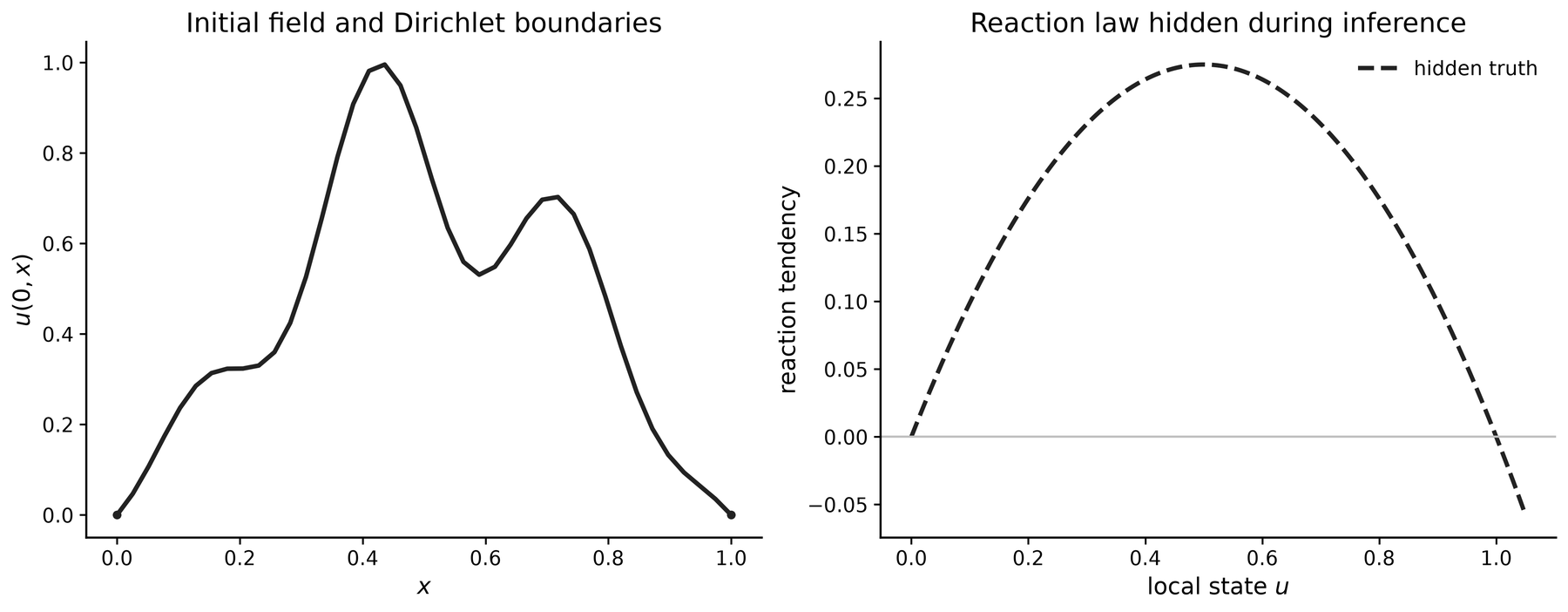
Consider the reaction–diffusion equation on \(x \in (0,1)\) with homogeneous Dirichlet conditions \(u(t,0) = u(t,1) = 0\):
\[\frac{\partial u}{\partial t}(t,x) = \nu\frac{\partial^2 u}{\partial x^2}(t,x) + c_\star(u(t,x)), \qquad c_\star(u) = r_\star u(1-u).\]
We assume that the diffusion term is known, but the logistic growth is hidden. We set \(\nu = 0.01\) and \(r_\star = 1.1\).
From a PDE to an ODE
Let \(x_i = ih\), exclude the two fixed boundary values from the state, and write \(\def\V#1{\boldsymbol{\mathbf{#1}}}\V{u}(t) = (u(t,x_1), \ldots, u(t,x_m))^\top\).
The centered finite-difference approximation
\(\frac{\partial^2 u}{\partial x^2}(t,x_i) \approx \frac{u(t,x_{i-1}) - 2u(t,x_i) + u(t,x_{i+1})}{h^2}\)
gives the method-of-lines ODE
\(\def\V#1{\boldsymbol{\mathbf{#1}}}\dot{\V{u}}(t) = \nu L_h \V{u}(t) + c(\V{u}(t)), \qquad L_h = \frac{1}{h^2}\operatorname{tridiag}(1, -2, 1).\)
This is now a differential equation we can use in dynestyx!
The Experiment
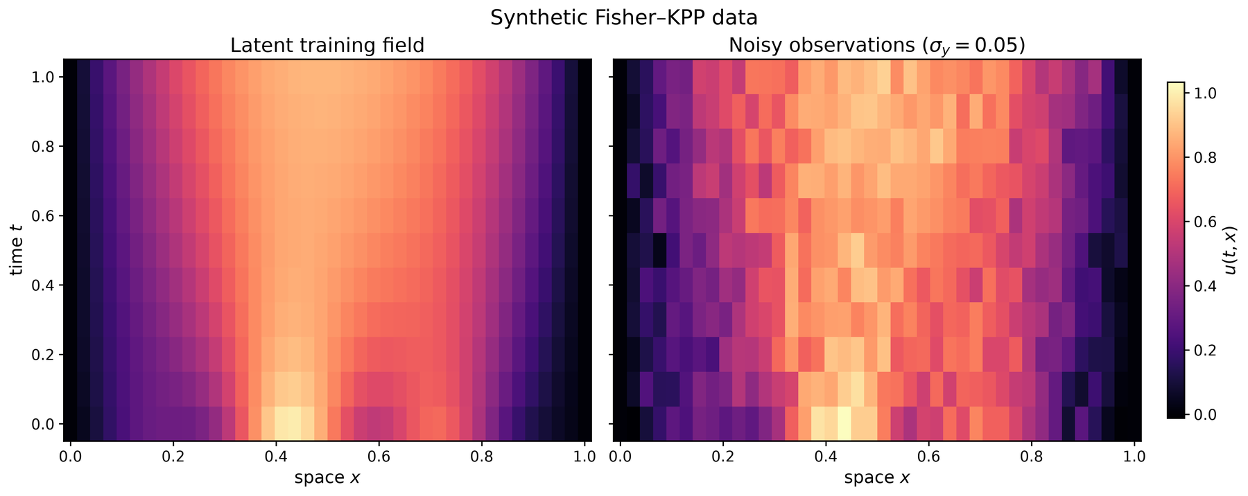
We use 40 grid points (including boundaries), and observe every interior node is observed every \(0.1\) time units with Gaussian noise of standard deviation \(0.05\).
Eleven fields from \(t = 0\) to \(t = 1\) are used for training; we then forecast from \(t = 1.1\) to \(t = 2.5\).
Three Candidate Reactions
The candidates mirror the ODE example:
\[\begin{aligned} c_{\mathrm{diffusion}}(u) &= 0, \\ c_{\mathrm{sparse}}(u) &= \beta_1 u + \beta_2 u^2 + \beta_3 u^3, \qquad \beta_j \sim \operatorname{Laplace}(0,1), \\ c_{\mathrm{HSGP}}(u) &= \mathrm{HSGP}(u). \end{aligned}\]
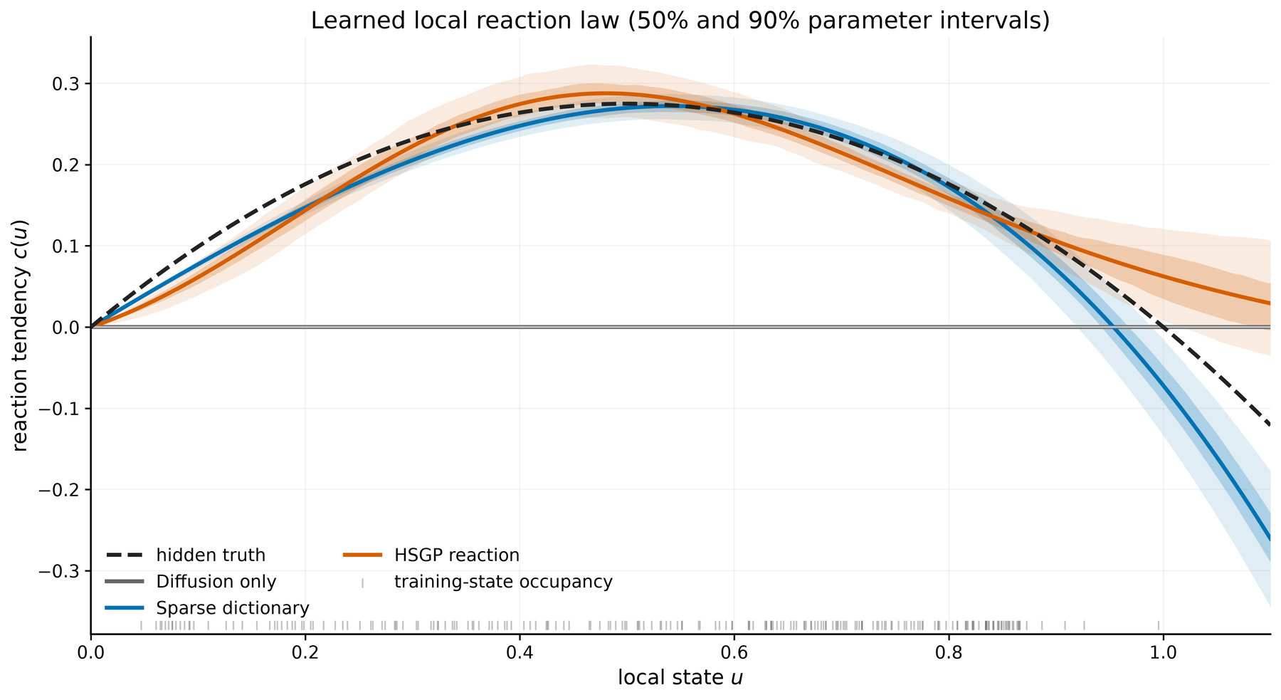
This is quite generous to the "sparse" solution, as the law really is quadratic!
We keep \(\nu\) known, and use the EnKF with SVI once again.
Reactions Are Learned Well
We recover the reactions well; on values during training, the reaction RMSE is \(0.2103\) for diffusion only, \(0.0190\) for the sparse dictionary, and \(0.0305\) for the HSGP.
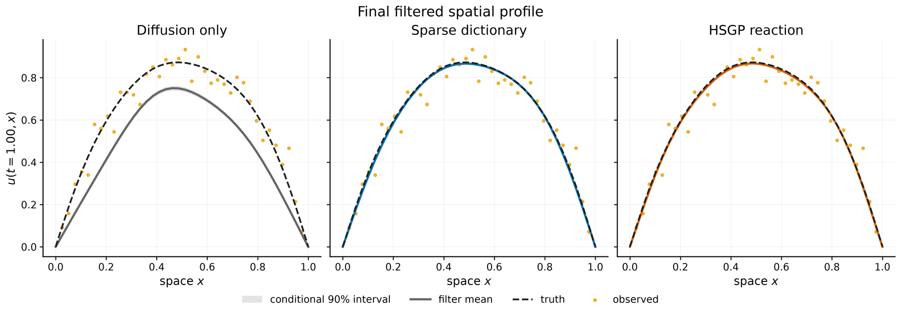
Filtered State Results
The filtered states show clearly that, despite informative results, the mis-specified model loses quickly. Hybrid models learn well.
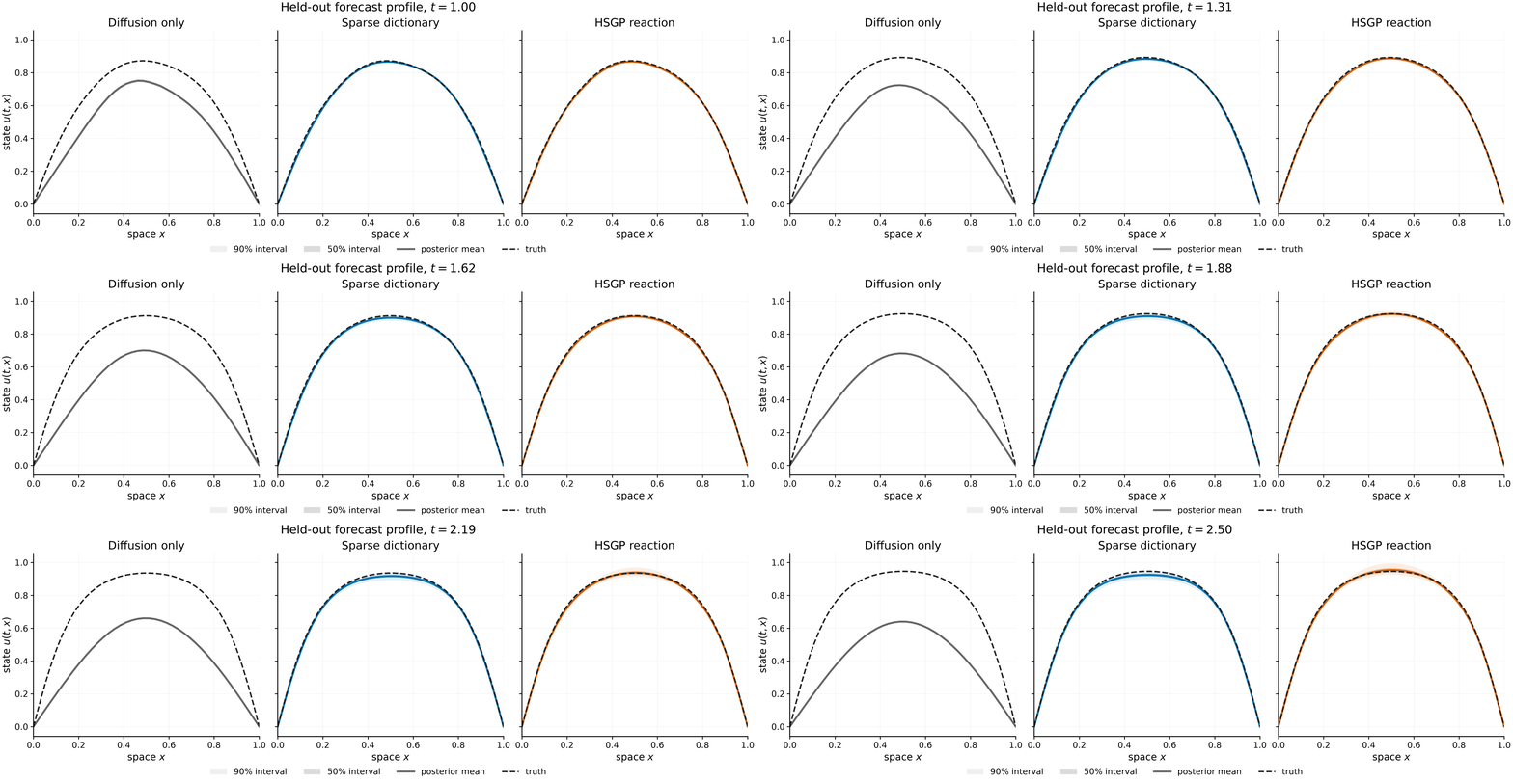
Forecasting Works Too
In forecasting using the learned reaction law, our hybrid models work quite well.
Summary and Lessons
- We presented a simple Bayesian recipe to deal with hybrid models.
- Two simple patterns: a sparse dictionary closure and GP closure, both work well in our toy examples.
- With
dynestyx, we showed how these models are simple to implement, and deal with things like missingness and differing inference methods. - We don't get perfect UQ here! Though we get much better than if we didn't try anything.
Open Problems and Future Work
- Our examples where quite simple here; let's get this to work on bigger and harder problems!
- We also had "easy" fixes to identifiability; how do we deal with this more generally?
- How far can we take the PDE formulation?
- What can we do for better calibration?
- How can we use generative methods (e.g., diffusion models) as part of this framework?
Questions?
danwaxman.github.io
dan@basis.ai
dynestyx

Paper

GitHub