GPs4SPs: Sequential Inference for Gaussian Processes in Signal Processing
Daniel Waxman
Basis Research Institute
Joint Work with Fernando Llorente and Petar Djurić
SIAM UQ 2026
March 25th, 2026

Gaussian Processes
Definitions and Intuitions
Computation Using Kernels
Model Selection
Gaussian Processes
Gaussian Processes: Definitions
Gaussian processes (GPs) are a flexible, non-parametric tool for Bayesian ML. [Rasmussen and Williams, MIT Press '05]
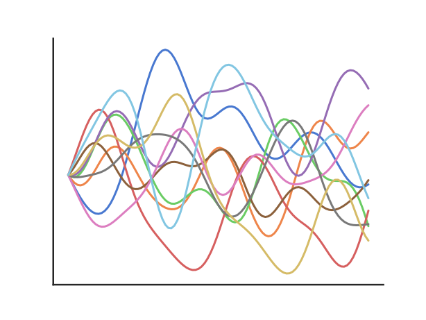
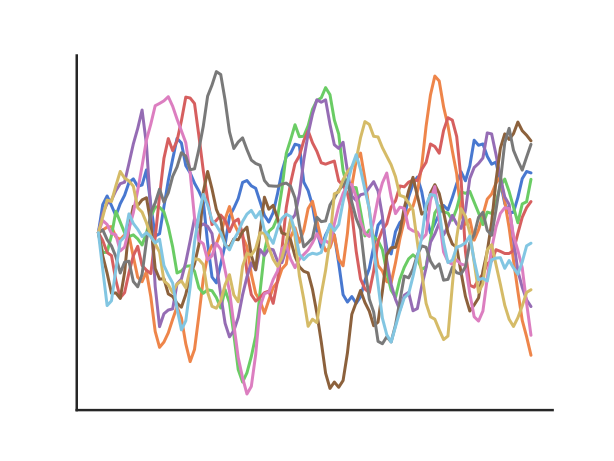
Basic Idea: A GP is a stochastic process \(f_t\) for \(t \in \mathcal{T}\) such the function evaluated at any set of points is jointly Gaussian.
A GP may then be specified by its mean function \( \mu(t) \) and covariance (or kernel) function \( k(t, t') \):
More ML-Like: the paths of any realization of a GP specify a prior over functions.
Gaussian Processes: Computation
In GP regression, we receive data \(t_i, y_i\), with \(i = 1, \ldots, n\), which are noisy observations of \(f(t)\).
\(f \sim \mathcal{GP}\!(0, k)\)
\(y = f(t) + \varepsilon\)
If \(\varepsilon\) is Gaussian, then the posterior is another GP. The posterior predictive is then
\(f_* \mid \mathcal{D} \sim \mathcal{N}(\mu_*, \sigma_*^2)\),
where the mean and the variance are given by
\(\mu_* = \mu(t_*) + k_{* \odot} K_{\odot \odot}^{-1} \delta\),
\(\sigma_*^2 = k(t_*, t_*) - k_{* \odot} K_{\odot \odot}^{-1} k_{* \odot}\).
Symbols
\([K_{\odot \odot}]_{ij} = k(t_i, t_j)\)Training Cross-Covariance
\([k_{* \odot}]_{i} = k(t_*, t_i)\)
Test Cross-Covariance
\(\delta = y - \mu(t)\)
Training Residuals
Gaussian Processes: Computation
In GP regression, we receive data \(t_i, y_i\), with \(i = 1, \ldots, n\), which are noisy observations of \(f(t)\).
\(f \sim \mathcal{GP}\!(0, k)\)
\(y = f(t) + \varepsilon\)
If \(\varepsilon\) is Gaussian, then the posterior is another GP. The posterior predictive is then
\(f_* \mid \mathcal{D} \sim \mathcal{N}(\mu_*, \sigma_*^2)\),
where the mean and the variance are given by
\(\mu_* = \mu(t_*) + k_{* \odot}\) \(K_{\odot \odot}^{-1}\) \(\delta\),
\(\sigma_*^2 = k(t_*, t_*) - k_{* \odot}\) \(K_{\odot \odot}^{-1}\) \(k_{* \odot}\).
Symbols
\([K_{\odot \odot}]_{ij} = k(t_i, t_j)\)Training Cross-Covariance
\([k_{* \odot}]_{i} = k(t_*, t_i)\)
Test Cross-Covariance
\(\delta = y - \mu(t)\)
Training Residuals
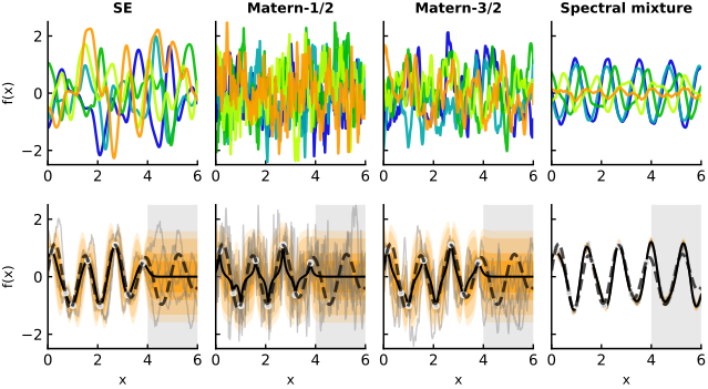
Gaussian Processes: Kernels
Gaussian Processes: Model Selection
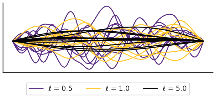
Even after specifying the form of \(\kappa(t, t')\), there are still many choices to be made.
In particular, each kernel comes with a set of hyperparameters which must also be selected.
The typical way to accomplish this with GPs is to maximize the marginal likelihood:
\(\log p(y | \theta) = \log \int p(y | f, \theta) p(f | \theta) \, df\)
Basic Idea: Choose priors that predict the data well.
The Trouble in Signal Processing
In signal processing, several challenges make the kernel approach for GPs difficult:
We're interested in inference over a very large time horizon \(T\).
We're interested in adaptive inference, i.e., in non-stationary environments.
Potentially, we're interested in online inference, i.e., in updating our model as we observe new data.
Sequential Learning for Gaussian Processes
Online Ensembles of GPs
Improvements From Filtering
Decentralized Solutions
Learning With Ensembles
To deal with the online learning problem, we'll pursue sequential ensembles.
There are two primary challenges here:
- How do we obtain closed-form updates for online learning?
- How do we adapt to non-stationary environments?
These are both difficult to accomplish with GPs in their conventional formulation. We'll address both by reformulating using a linear-Gaussian approximation of GPs.
How Linearization Helps
The point here is that, under a linear-Gaussian approximation to a GP, we can continue with Kalman filtering updates.
The resulting models are generally known as
To obtain the online ensemble of basis expansions (OEBE), we can additionally combine with OBS or O-BMA.
Random Fourier Features
One popular approximation for stationary GPs are Random Fourier Features (RFF) [Rahimi and Recht, NeurIPS '07].
These features are derived by a Monte Carlo approximation of the Wiener-Khinchin integral
\(\kappa(t, t') = \int_{\mathbb{R}^d} \exp(2\pi i s^\top (t - t')) \, dS(s),\)
where \(S(s)\) is a spectral density and \(i\) is the imaginary unit.
The resulting basis expansion is given by sampling \(F / 2\) spectral frequencies, \(s_1, \dots, s_{F/2}\), and computing the features
\(\phi(x) = \left[ \cos(2\pi s_1^\top x), \sin(2\pi s_1^\top x) \cdots \cos(2\pi s_{F/2}^\top x), \sin(2\pi s_{F/2}^\top x) \right].\)
Hilbert Space Gaussian Processes
RFF, while simple, suffers harshly from the curse of dimensionality.
Hilbert Space Gaussian Processes (HSGP) [Solin & Sarkka, S&C '20'] address this by instead deriving a quadrature rule over the Wiener-Khinchin integral.
For scalar GPs on \([-L, L]\), the corresponding basis function is
\( \phi_k(t) = S\left(\frac{k\pi}{2L}\right) \frac{\sin\left((k\pi(t+L) / 2L)\right)}{\sqrt{L}}, \quad k = 1, \dots, F. ,\)
where \(S(s)\) is a spectral density.
Corresponding approximations in higher dimensions are possible but expensive. We instead pursue additive HSGP approximations, which writes \(f(x) = \sum_{d=1}^D f_d(x_d)\).
Bayesian Model Averaging
To cope with hyperparameters in online settings, we'll use ensembles.
Bayesian model averaging (BMA) is the most common approach to linear weighting.
BMA weighs each model according to its
\(w_i = \mathrm{Pr}(M_i | \mathcal{D}) = \frac{p(M_i | \mathcal{D}) p(M_i)}{\sum_{j=1}^K p(M_j | \mathcal{D}) p(M_j)}\).
In the online setting, we obtain recursive weights via the prequential decomposition of the log-likelihood:
\(w_{t+1,k}^{\text{BMA}} = \frac{ w_{t, k} p_k(y_{t+1} | \mathbf{x}_{t+1}, \mathcal{D}_t)}{\sum_k w_{t, k} p_k(y_{t+1} | \mathbf{x}_{t+1}, \mathcal{D}_t)}\).
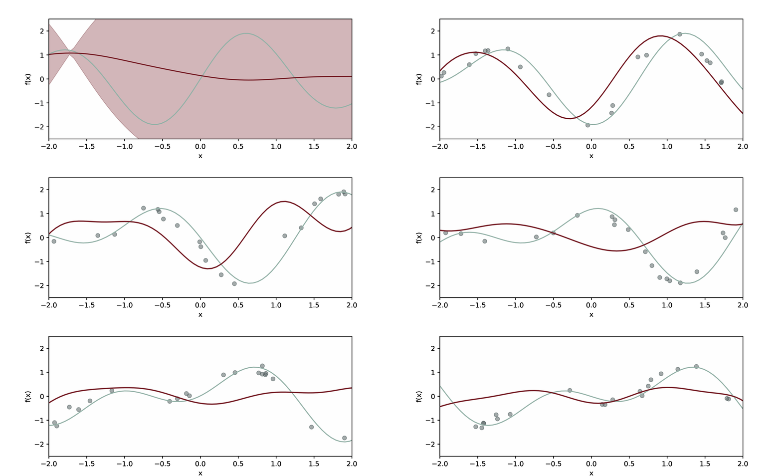
But What About Dynamic Problems?
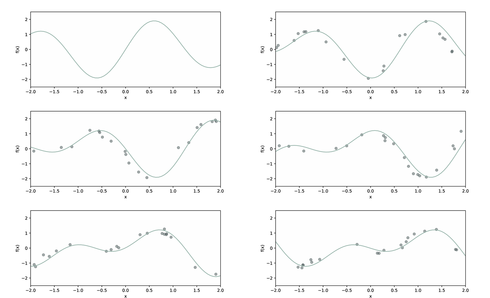
OEBE Fails at Dynamic Problems
Solution: Parameter Random Walk
From the filtering perspective, a random walk on parameters is an obvious choice.
In particular, with a Gaussian random walk, we maintain exact Kalman filter updates.
We adapt a hyperparameter \(\sigma_\text{rw}^2\), and the state-space model
\( \theta_{t+1}^{(m)} = \theta_t^{(m)} + \varepsilon_{\text{rw}}^{(m)}, \)
and observation model
\( y^{(m)} = \phi^{(m)}(x)^\top \theta_t^{(m)} + \varepsilon_{t}^{(m)}. \)
We call the resulting model a distributed online ensemble of basis expansions (DOEBE) [DW & Djurić, TMLR '24].
DOEBE Solves the Dynamic Problems
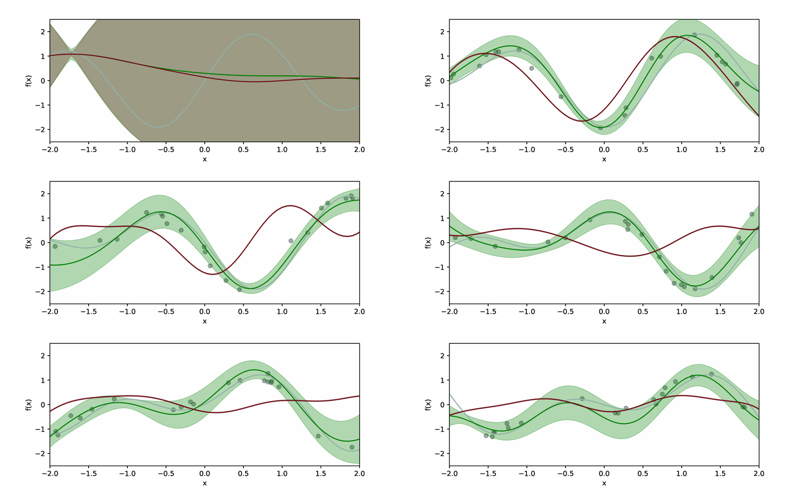
DOEBE Solves the Dynamic Problems
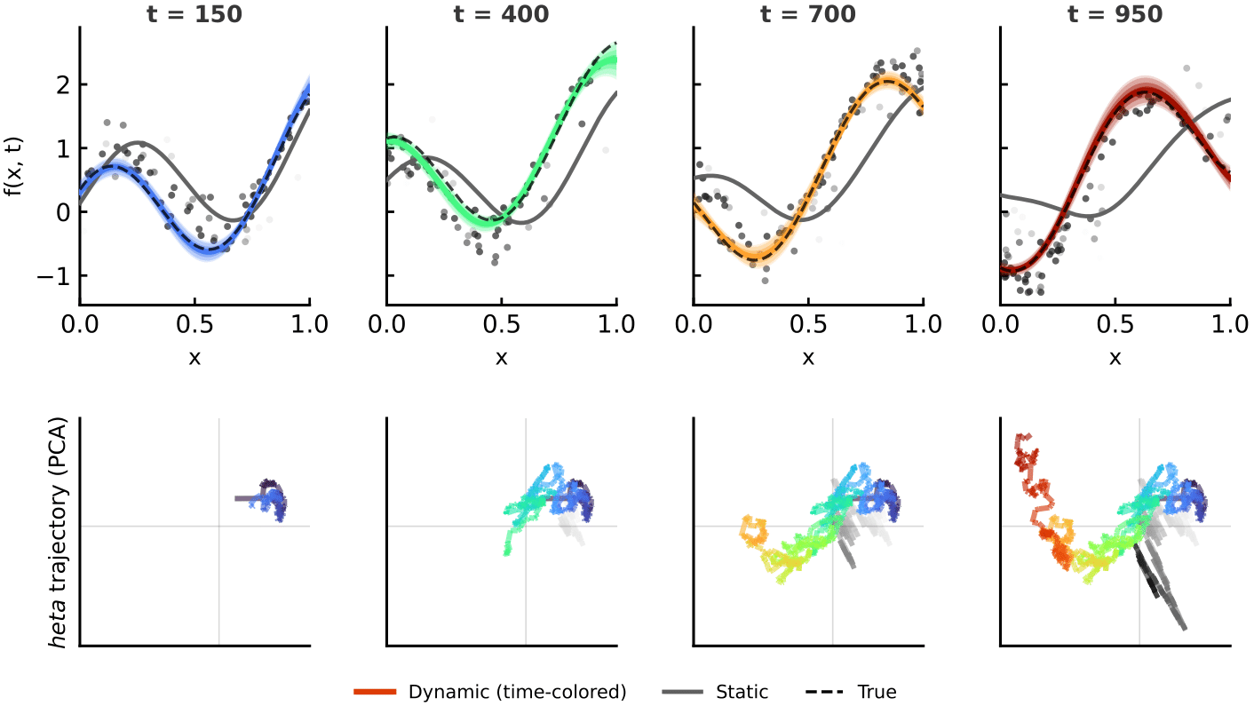
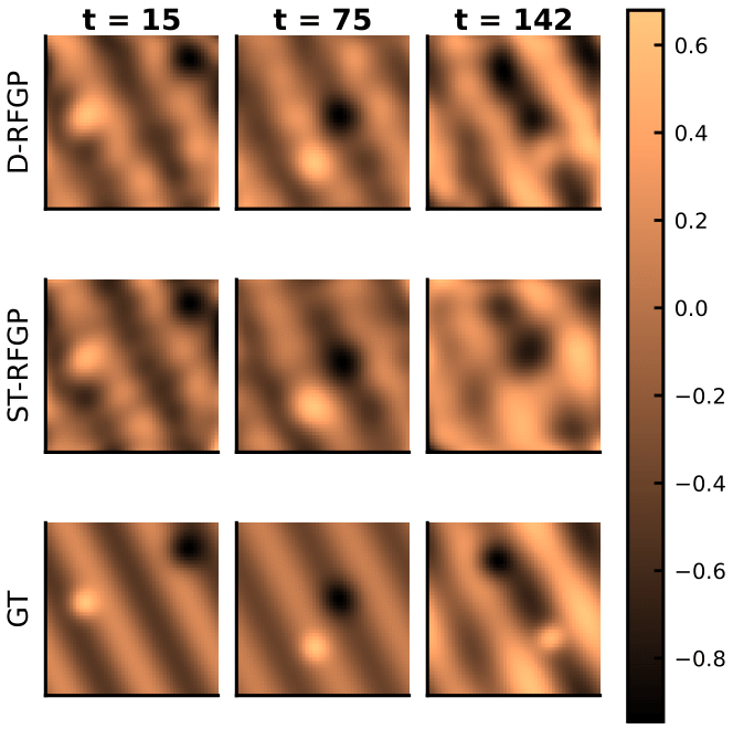
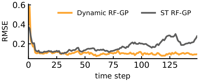
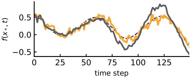
Alternative Approach: Spatiotemporal Kernels
An alternative, intuitive approach is to use a spatiotemporal kernel, e.g.,
\( \kappa(t, t') = \kappa_t(t, t') \kappa_s(x, x'). \)
This works well in limited problems, but deteriorates as the time horizon grows.
DOEBE Solves the Dynamic Problems
Extensibility Through Filtering Theory
What we've just done is (1) approximate the GP as a linear state-space model, and (2) use standard Gaussian filtering.
The core thesis of this talk: we're doing filtering already, let's figure out new extensions!
We'll talk about two extensions: decentralized inference and robust inference.
Motivation & Setting
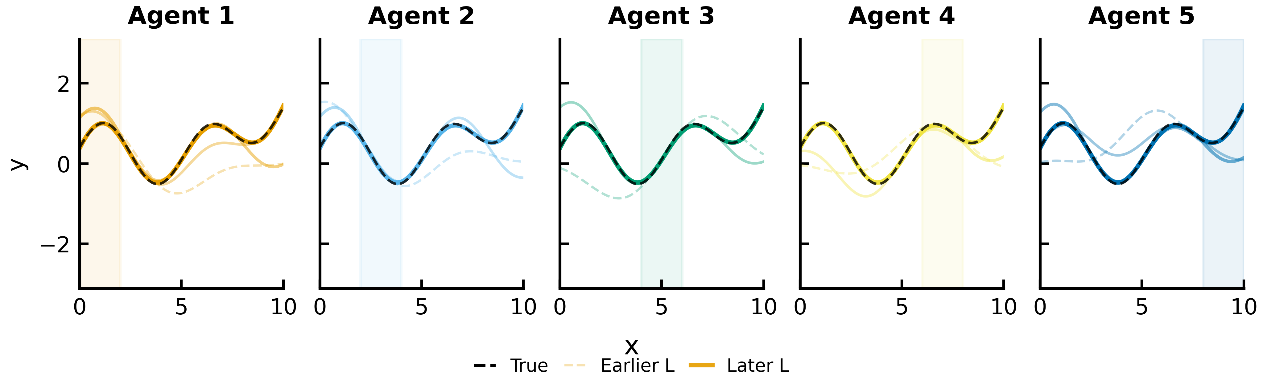
We study a decentralized, online multi-agent regression problem.
- Estimate a function \(f: X \to Y\) by combining the estimates of multiple agents.
- Data arrives online: agent \(A_n\) receives \((x_{n,t}, y_{n,t})\) at time \(t \in \{1, \ldots, T\}\).
- Agents communicate only with neighbors in a weakly connected graph \(\mathcal{G} = \{\mathcal{N}, \mathcal{E}\}\).
- Inference should be collaborative and decentralized, without a permanent fusion center.
We model \(f\) with Gaussian processes (GPs), then adapt the resulting filtering updates to the multi-agent setting.
Contributions
We give the first GP-based method for the decentralized, online multi-agent setting [Llorente*, DW*, & Djurić, ICASSP 2025].
With relatively small communication overhead, our method closely matches the centralized posterior.
In the limit of sufficient computation, it recovers the centralized result exactly.
This gives a method that is simultaneously distributed, Bayesian, online, and asymptotically exact.
Using a Fusion Center
Let us begin with a distributed approach using a fusion center.
We will then move to a decentralized version.
Our approach works by combining subposteriors, i.e., the posterior of each local agent.
In linear-Gaussian settings, these updates are additive in the information quantities:
\[ \mathbf{P}_{n,t} = \frac{1}{\sigma_{obs}^2}\Phi_{n,t}\,\Phi_{n,t}^{\top} \qquad \mathbf{s}_{n,t} = \frac{1}{\sigma_{obs}^2}\Phi_{n,t}\,y_{n,t} \]
Using a Fusion Center
In linear-Gaussian settings, these updates are additive in the information quantities:
\[ \mathbf{P}_{n,t} = \frac{1}{\sigma_{obs}^2}\Phi_{n,t}\,\Phi_{n,t}^{\top} \qquad \mathbf{s}_{n,t} = \frac{1}{\sigma_{obs}^2}\Phi_{n,t}\,y_{n,t} \]
This results in posterior information quantities
\[ \mathbf{D}_{c,t} = \sum_{\tau=0}^{t} \sum_{n=1}^{N} \mathbf{P}_{n,\tau} = \sum_{n=1}^{N} \mathbf{D}_{n,t} \qquad \eta_{c,t} = \sum_{\tau=0}^{t} \sum_{n=1}^{N} \mathbf{s}_{n,\tau} = \sum_{n=1}^{N} \eta_{n,t} \]
Additive Consensus
Given local quantities \(\mathbf{a}_1, \ldots, \mathbf{a}_N\), additive consensus is an iterative procedure that allows agents to all converge to the sum \(\mathbf{a}_1 + \cdots + \mathbf{a}_N\) communicating only to their neighbors.
This works by taking local averages, multiplying them by the total number of agents at the end.
Even for directed graphs, additive consensus converges to the correct quantity.
Decentralized Learning
For decentralized learning, i.e., without a fusion center, we use additive consensus.
We thus proceed with \(L\) steps of additive consensus, before updating the posterior.
For simplicity, we use equal weighting:
\[ \tilde{\mathbf{P}}_{n,t}^{(\ell+1)} = \frac{1}{N_n + 1}\left(\tilde{\mathbf{P}}_{n,t}^{(\ell)} + \sum_{j \in \mathcal{N}_n}\tilde{\mathbf{P}}_{j,t}^{(\ell)}\right), \]
\[ \tilde{\mathbf{s}}_{n,t}^{(\ell+1)} = \frac{1}{N_n + 1}\left(\tilde{\mathbf{s}}_{n,t}^{(\ell)} + \sum_{j \in \mathcal{N}_n}\tilde{\mathbf{s}}_{j,t}^{(\ell)}\right). \]
Online Ensembles with Approximate BMA
As discussed before, one trend is using BMA to ensemble GP models:
\[ w_{t+1}^{(m)} \propto p(y_{t+1}\mid x_{t+1})w_t^{(m)} \]
In the decentralized setting, this is difficult, since we must estimate the marginal likelihood.
We introduce two variants of decentralized online BMA:
- Local BMA, where online BMA is performed on local data only;
- Independent Consensus BMA, where BMA is performed via an independence approximation.
Illustration
Experimental Baselines and Setup
We perform our experiments against several different baselines:
- NPAE [Kontoudis & Stillwell, ICRA 2021], an offline method for distributed GP inference;
- DOMKL [Hong & Chae, TNNLS 2021], a frequentist distributed multiple online kernel method;
- AdaRaker [Shen et al., JMLR 2019], a frequentist online multiple kernel method; and
- SVI GPs [Hensman et al., UAI 2013], an efficient offline GP method.
For all experiments, we use \(L = 10\) iterations with \(N = 5\) agents and \(M = 3\) models. RF-GP methods used \(J = 50\) random features.
Experiment Results
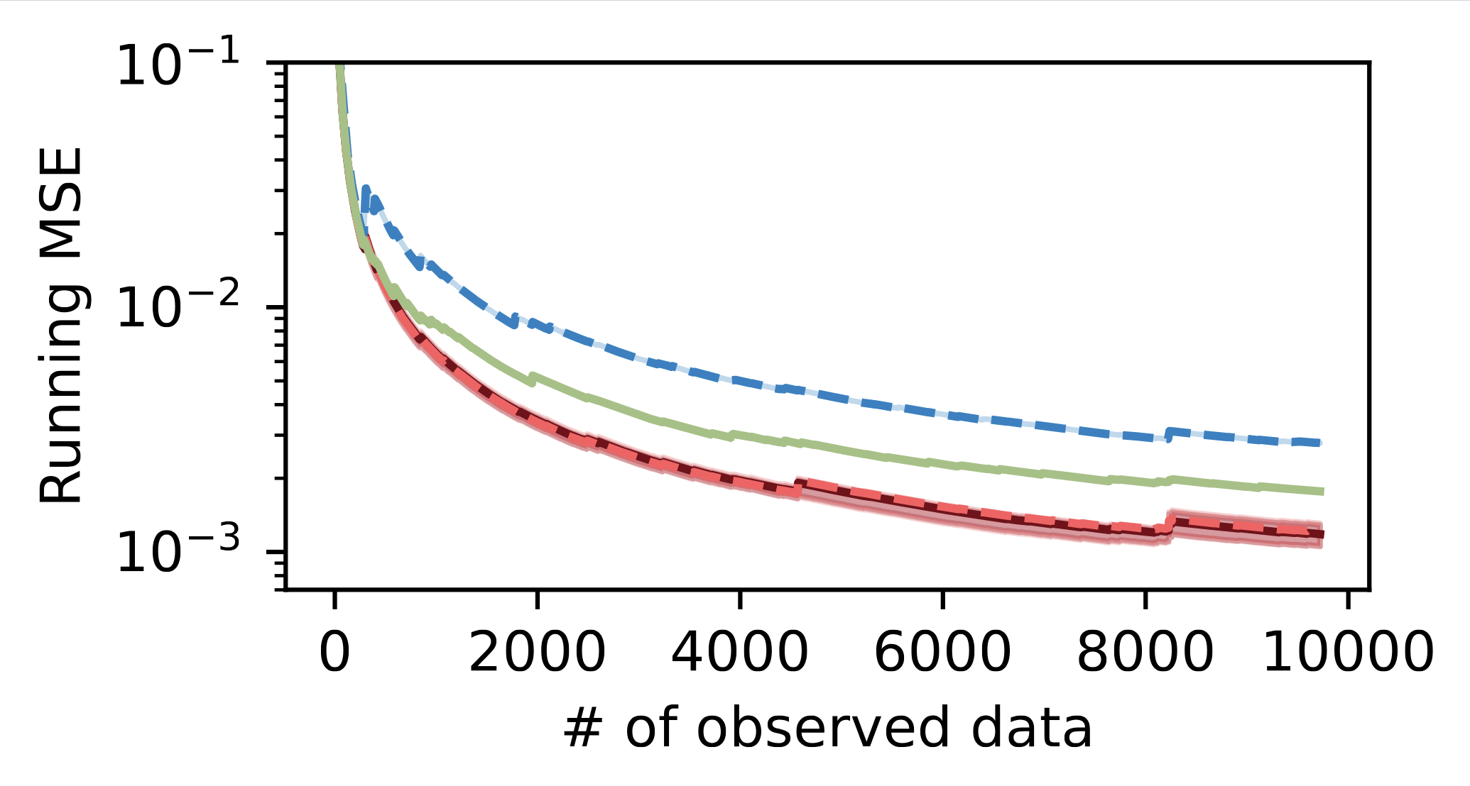
Running MSE
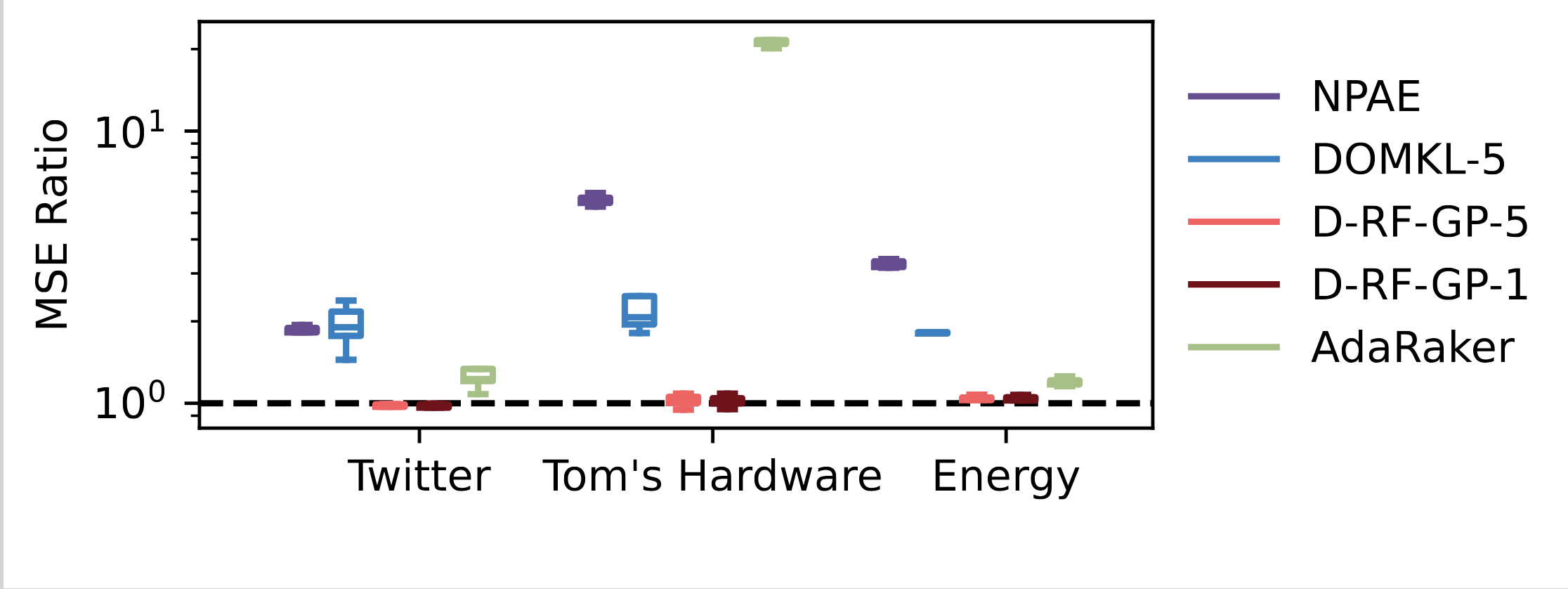
MSE on Holdout Data
Takeaways
- Our method beats all presented baselines, even offline and centralized ones.
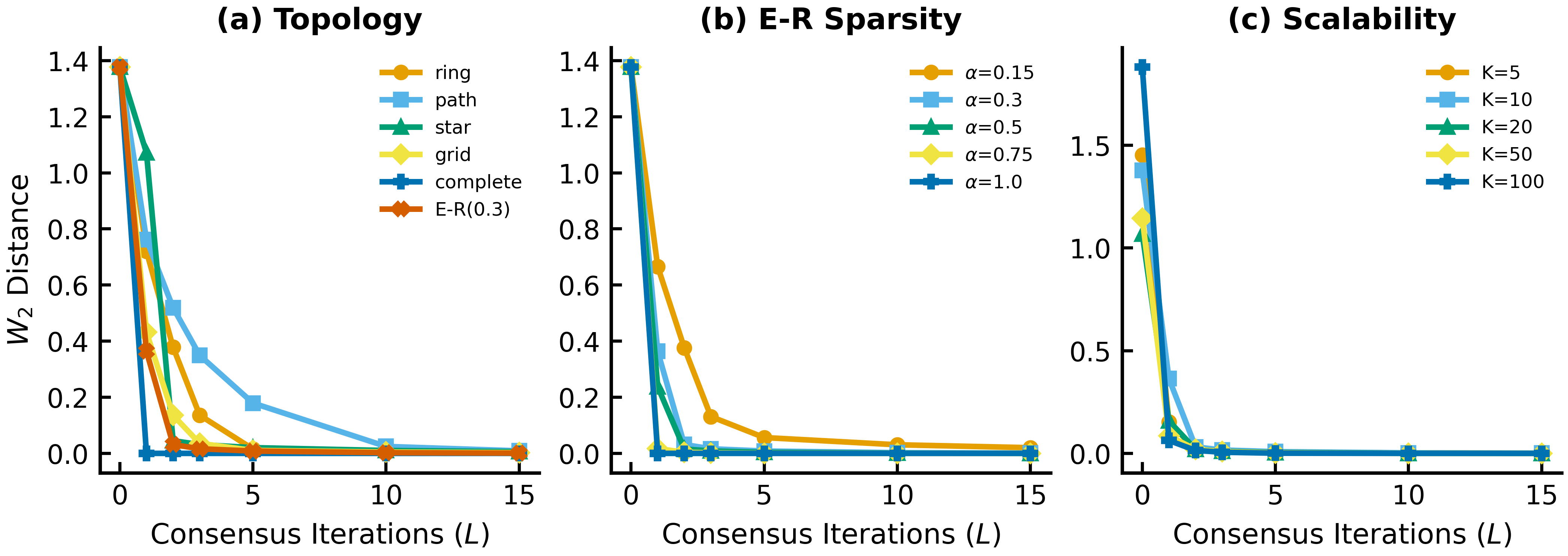
- Consensus performs well in these experiments, with \(N = 1\) and \(N = 5\) agents performing similarly well.
- On the datasets presented, the ensemble of RF-GPs performs similarly to SVI GPs, a gold standard of GP inference.
Consensus Converges Quickly
Robust Gaussian Processes
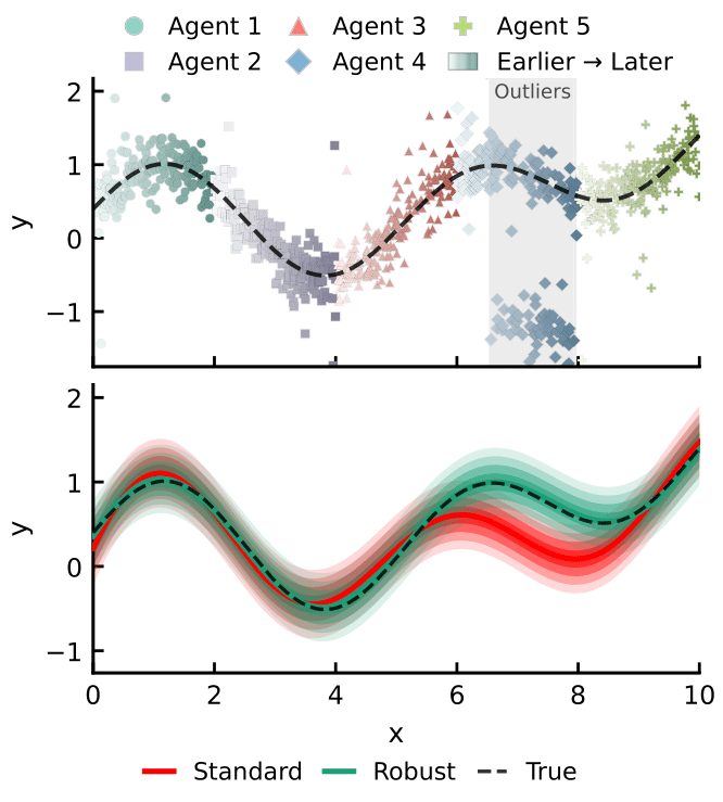
One additional thing we get "for free" is robust inference, from the well-explored robust Kalman filtering literature.
This is useful for, e.g., when one or more agents are faulty or adversarial, as Gaussians are sensitive to large errors.
We can combine this with GPs, and even decentralized GPs! [Llorente et al. (including DW), ICASSP 2026].
Robust Information Filtering
In a robust distributed information filter, each agent forms a diagonal weight matrix \(\mathbf{W}_{k,t} = \operatorname{diag}(w_{k,t}^{(i)})\).
Each weight \(w_{k,t}^{(i)}\) is a function of the standardized residual \[ e_{k,t}^{(i)} = \frac{y_{k,t}^{(i)} - \hat{y}_{k,t}^{(i)}}{\sigma_{y,k,t}}, \] so atypical observations are downweighted.
The information-form updates become weighted sums:
\[ \mathbf{D}_t \leftarrow \mathbf{D}_{t-1} + \sum_k \frac{\Phi_{k,t}^{\top}\mathbf{W}_{k,t}\Phi_{k,t}}{\sigma_{obs}^2}, \qquad \eta_t \leftarrow \eta_{t-1} + \sum_k \frac{\Phi_{k,t}^{\top}\mathbf{W}_{k,t}y_{k,t}}{\sigma_{obs}^2}. \]
Equivalently, this is inference under a tempered likelihood that reduces the influence of outliers.
Example Weighting Schemes
Robust weights are chosen from weighting functions that shrink or reject large residuals.
Huber weighting keeps full weight for small residuals and decays like \(1/|e|\) once \(|e| > \delta\): \[ w_{\mathrm{Huber}}(e) = \begin{cases} 1, & |e| \le \delta,\\ \delta / |e|, & |e| > \delta. \end{cases} \]
Hampel weighting uses three thresholds \(a < b < c\): full weight near zero, gradual downweighting for moderate residuals, and zero weight for very large residuals.
These schemes let us trade off stability against aggressiveness in rejecting corrupted data.
Robust GP in Action
Sequential Learning for Gaussian Processes
SDEs
Markovian GPs
Improvements From Filtering
Stochastic Differential Equations
Let us define an SDE over \(\bar{f}\),
\(\bar{f}_t\) \(= F(\bar{f}, t) \, dt\) \(+ L(\bar{f}, t) \, d\beta\).
In the special case where \(F(\bar{f}, t)\) is a linear function of \(\bar{f}\) and \(L\) is constant, we obtain a linear SDE.
If we observe \(y(t) = H \bar{f}(t) + \epsilon(t)\), where \(\epsilon(t)\) is Gaussian noise, we may obtain filtering and posterior solutions for \(\bar{f}(t)\) with Kalman(-Bucy) filtering/smoothing.
Markovian Gaussian Processes
Some GPs (which we call Markovian GPs) can be represented as a linear SDE, where \(\bar{f}\) contains \(f(t)\) and some derivatives, chosen to match the GP prior [Sarkka et al, SP Mag, '13].
The discretized state space representation allows for posterior inference in linear time.
Extensions From Filtering Theory
- Just as in the linearized GP case, we can obtain stronger results via stronger filtering theory.
- One example is in robustness.
- Lintel uses classical rejection Kalman filtering to get robust inference [DW & Djurić, FUSION 2024].
- More generally, generalized Bayesian techniques have been used, which correspond exactly to robust Kalman smoothing [Laplante et al., ICML 2025].
- Another example is in non-Gaussian observations.
- A principal example here is iterated posterior linearization [García-Fernández et al., SPL 2019].
Conclusions
Signal processing requires scalable solutions, linear in \(T\), and often online.
The machine learning literature has developed such methods. They're all some sort of classical filter.
By recognizing this, we get cool extensions "for free," and can also work towards better approximations.
Two approaches we explored were in linearization and Markovian GPs, but variational/EP approximations also admit nice SP-based interpretations.